E.  Aggregate Model of the Macro Economy

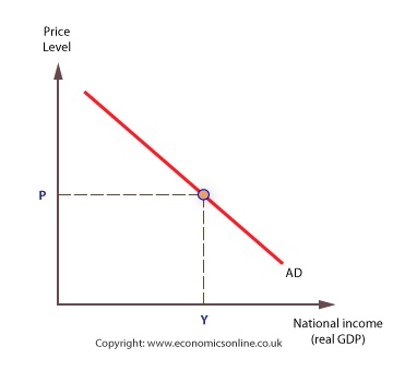
1.  Aggregate demand curve

• Shows combinations of the price level (P) and real income or GDP (Y) that result in simultaneous equilibriums in both the goods and money markets

• Based on the different types of expenditures (C, I, G, and X - M)

a.  Graph

b.  Shifting the aggregate demand curve

•  Anything affecting the individual components of expenditures will affect the AD curve

.

(1)  Factors affecting the aggregate demand curve

C = f [T_P(-), r (-), CC (+), W (+), CR (+), DB (-)]

I = f [r (-), T_B(-), PR (+), CU (+)]

G = f [G (+)]

(X - M) = f [Y* (+), R (-)]

.

AD = f [T_P(-), r (-), CC (+), W (+), CR (+), DB (-), T_B(-), PR (+), CU (+), G, Y* (+), R (-)]

.

(2) Monetary policy

• Use money supply and interest rates to affect economy

MS increases => r decreases => C, I increases => AD increases

MS decreases => r increases => C, I decreases => AD decreases

.

(3) Fiscal policy

• Use government spending and / or tax changes to affect economy

G increases => AD increases

G decreases => AD decreases

.

T_P increases => C decreases => AD decreases

T_P decreases => C increases => AD increases

.

T_B increases => I decreases => AD decreases

T_B decreases => I increases => AD increases

.

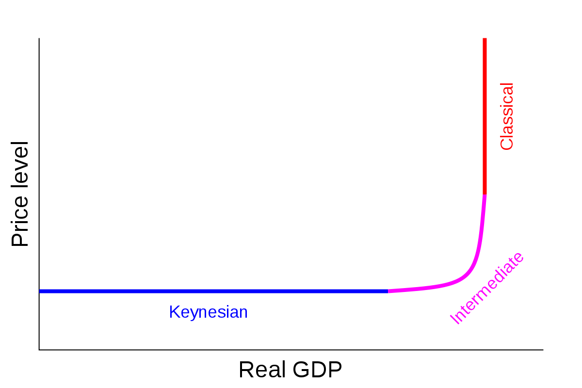
2.  Aggregate supply curve

• Shows the price level at which firms are willing to produce different amounts of real goods and services

• Depends on quantity and quality of resources used in production, efficiency with which resources are used, and production technology

.

a.  Short-run aggregate supply

• Amount of resources, efficiency of their use, and level of technology constant in short-run

• Affected only by changes in the prices of inputs

.

.

b.  Long-run aggregate supply

• Potential output - full-employment level of output

• Maximum amount that can be produced, given resources and technology available

.

.

3.  Equilibrium

.

.

.

.

.

.

.

.

.

.

4.  Changes

a.  Aggregate demand

.

.

.

.

.

.

.

.

.

.

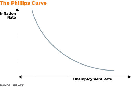
(1)  Phillips curve

• Shows relationship between inflation and unemployment

• Inverse relationship

.

(2)  Using policy to affect the economy

(a)  Monetary policy

• To counteract a downturn:  increase money supply => decrease interest rates

• To counteract overheating:  decrease money supply => increase interest rates

.

.

.

.

.

.

.

.

.

.

• Effectiveness of monetary policy

- Depends on responsiveness of expenditures to changes in interest rates

.

.

.

.

.

.

.

.

.

.

(b)  Fiscal policy

• To counteract a downturn:  increase government expenditures, decrease taxes

• To counteract overheating:  decrease government expenditures, increase taxes

.

.

.

.

.

.

.

.

.

.

• Budget deficit and the national debt

- Deficit if government expenditures > government revenue

- Debt = accumulated deficits

- Are deficits and debt a problem?

i)  Crowding out

.

.

.

.

.

.

.

.

.

.

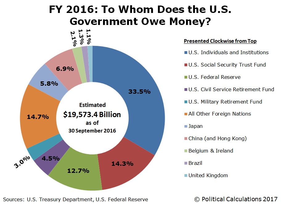
ii)  Who owns the debt?

.

iii)  Is the debt a burden on future generations?

• Depends on how it it used now

• Future generations can borrow to push debt into future

• Problem if more productive private sector investments are crowded out

.

(c)  Lags

• Takes time for policy to take effect

- Recognize problem

- Implement policy

- Have impact on problem

• Recognition lag similar for both monetary and fiscal policy

• Implementation lag longer with fiscal policy - need to pass legislation, implement legislation

• Impact lag longer with monetary policy - indirect impact on economy

 .

b.  Short-run aggregate supply

.

.

.

.

.

.

.

.

.

.

• Stagflation - combination of both unemployment and inflation

• Difficult to counteract with policy

.

c.  Long-run aggregate supply

• Leads to long-term economic growth

.

.

.

.

.

.

.

.

.

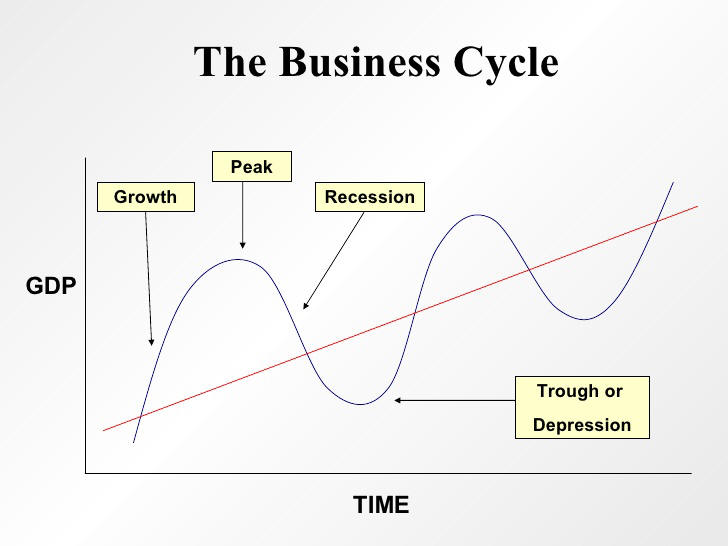
5.  Business cycle

• Expansion - increase in economic activity

• Recession - decrease in economic activity

.

a.  Economic indicators

(1)  Concurrent indicators

• Move along with the economy

- Employees on nonagricultural payrolls
- Personal income less transfers
- Industrial production
- Manufacturing and trade sales

.

(2)  Leading indicators

• Move in advance of the economy

- Average weekly hours, manufacturing
- Average weekly initial claims for unemployment insurance
- Manufacturer's new orders, consumer goods and materials
- Institute for Supply Management new orders index
- Manufacturer's new orders, nondefense capital goods excluding aircraft
- Building permits, new private housing units
- Stock prices, 500 common stocks
- Leading Credit Index
- Interest rate spread, 10-year Treasury bond less federal funds
- Average consumer expectations for business and economic conditions

.

(3)  Lagging indicators

• Move after the economy moves

- Average duration of unemployment
- Inventories to sales ratio, manufacturing and trade
- Labor cost per unit of output, manufacturing
- Average prime rate
- Commercial and industrial loans
- Consumer installment credit to personal income ratio
- Consumer price index for services

• Calculated by the Conference Board

.

b.  Impact on managerial decisions

• Demand affected through impact on income

• More intense competition for market share and profits