In our first spectroscopic experiment of the semester we examine thermal radiation radiation from two familiar radiators: the sun, and a garden variety light bulb. The Sun is the hottest blackbody radiator in the local neighborhood of the earth, and a light bulb is the easiest blackbody radiator we can readily control in the lab. We'll examine these in turn. Our goal is to use Planck's Law radiation curve to answer two questions. Using light from the sun, we ask: how big (or small) is the new universal constant, $h$, Planck's constant, in terms of orders of magnitude. What can solar radiation tell us about that? The other research question is this: using incandescent light, what is the temperature of a light bulb?
Perhaps after this lab we will begin to usefully doubt our eyes. `Seeing is believing', it is said, but first we must be sure of the detector characteristics of our own eyes?
Figure 1. My new hobby, teaching answers to tricky questions posed by scientist trying stump other scientists through tricky questions taught to their children (of the scientists who are the intended targets of the tricky questions.....)
4.1.2 Historical background stuff that I cannot keep myself from observing. You might not need to read it, but,....
Blackbody radiation was the subject which led to the quantum revolution, a crisis in physics from which we have still not recovered. Quantum theory arose not because of
the quantization of matter, but rather because of the quantization of light. It really is true, as G.P. Thomson once said [1] that it is ``...seldom that a scientific conception is born in its final form, or owns a single parent. More often it is the product of a series of minds, each in turn modifying the ideas of those that came before, and providing material for those that come after.'' The notion of the quantum of radiation had a number of prominent refiners, Einstein chief among them, but the idea had just one parent, Max Planck.
Studies performed by the pre-quantum scientists of the 19th Century, of heat radiation intensity data showed that the wavelength corresponding to the peak of the radiation intensity shortened inversely with temperature, \begin{equation}
\lambda_{max} T = 2.898 \times10^{-3} m \cdot K, \end{equation} a relation known as Wein's displacement law
and that total energy radiated, integrated over all wavelengths, was proportional to the fourth power of the temperature \begin{equation}
\int_o^{\infty} \rho(\lambda) d\lambda = 5.67 \times 10^{-8}T^4,\end{equation} known as the Stefan-Boltzmann law, where the constant where the constant (the Stefan-Boltzmann constant) has units of $ W/(m^2 K^4)$. But the constants had no basis in theory for Planck's predecessors. Worse, the best of classical conceptions held that radiation law applying to cavity radiation (the best approximation of an ideal blackbody radiator), was \begin{equation}
\rho_{\nu} d\nu = \frac{8\pi \nu^2 k_B T}{c^3} d\nu, \end{equation}
known as the Rayleigh-Jeans law, which used the equipartition theorem to assign and average energy of $k_BT$ to each cavity mode (standing wave) for which the number of modes per unit volume, per unit frequency was known to be $8\pi \nu^2 d\nu/c^3$. Brilliant, and nicely in agreement with the data in the long wavelength limit, but it was horribly wrong in the short wavelength limit. (The radiant power increases without limit at short wavelength-even a room temperature object should be able to melt things, all things, in its vicinity from the short wavelength heat radiation, theoretically , that is. Well, the theory was scandalously wrong--the ultraviolet catastrophe, it was eventually called. There see, I'm doing it again! I am lending credence to a myth often found in texts. The logical sequence of events was not the historical one, Planck was not motivated to solve this problem as it didn't exist for him. His great dilemma was whether to take the leap and posit that light energy is exchanged with what he called the material (atomic) 'resonators', individually, in discrete chunks or not. Later he called it an act of desperation...I gotta track down that reference...see, I'm doing it again....using memory rather than references...so unscholarly....sheesh.
Enter Planck. The theoretical solution to this problem was first derived by him in 1900, and finally understood by him in 1909, suggested that idealized model oscillators within the material walls absorb and emit radiation in quantum jumps of discrete bundles of energy in the amount
$\epsilon = h\nu$, It was a radical departure from classical concepts. Planck held that the energy of the bundle was proportional to its frequency rather than the amplitude of the electromagnetic wave. This left a constant of proportionality to be determined by fitting data for various black body curves. The constant is a universal constant and is now called Planck's constant, $h = 6.626 \times 10^{-34} J-sec$.
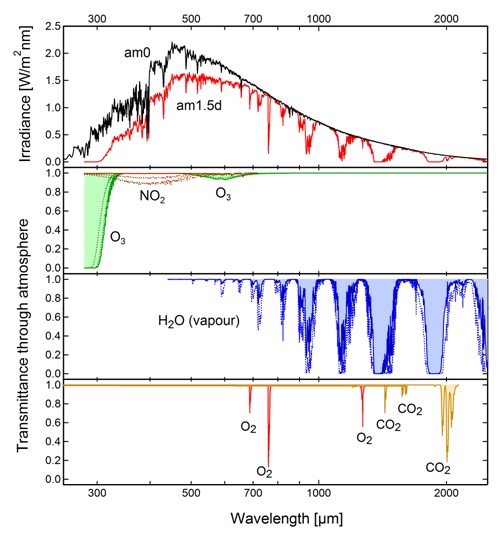
Figure 2, A comparison of the AMO and AM1-5d spectrum, indicating sources of absorption in the earth's atmosphere, and on the bottom, The AM0 spectrum (black line) vs blackbody radiation at 4550 K, 5775 K and 6500 K.
In Planck's theory, the distribution of heat radiation, that is, of electromagnetic energy, per unit volume, per unit frequency, that would be in equilibrium with the oscillators in the surface of the material at temperature $T$ was
\begin{equation}
\rho_{\nu} d\nu= \frac{8\pi h \nu^3}{c^3}\frac{1}{e^{h\nu/k_BT} -1}d\nu, \end{equation}
or, expressed as a function of wavelength
\begin{equation}
\rho_{\lambda}d\lambda = \frac{8\pi c h }{\lambda^5}\frac{1}{e^{hc/\lambda k_BT} -1}d\lambda. \end{equation}
Comparing our data with {\em a version } of this latter expression of Planck's energy distribution, since our data is obtained experimentally as a function of wavelength is the principle part of the experiment.
For use in modeling our data, we will restate $\rho_{\lambda}$ using constants with a view to using data to help us get a feel for the new universal (quantum) constant $h$,
\begin{equation}
\rho_{\lambda}d\lambda = \frac{C_1 }{\lambda^5}\frac{1}{e^{C_2/\lambda T} -1}d\lambda, \end{equation}
by adjusting the value of $C_1$ to adjust the amplitude of the theory curve to fit the data, and $C_2$ to fit the peak and the shape of the theory curve to the best fit the data. The constant $C_2 = hc/k_B$, according Planck's theory, which has a value of $1.439 \times 10^{ -2} m \cdot K$. The Ocean Optics spectrometer (see figure 3 below) however furnishes wavelength data in units of nm, and so the value of this constant in those units would be $10^9$ times bigger (think about this!), $1.439 \times 10^7 nm \cdot K$.
There are of course non-idealities associated with real blackbody radiators that are not a part of Planck's model. But the model did more than explain simple blackbody radiation curves- it contributed new ideas to the stock of concepts used to understand the physical universe, concepts of over arching importance, concepts very much at variance with the previously existing stock of those describing electromagnetic radiation, still then quite new. And when the observed notches in the solar blackbody spectrum were looked at with high resolving power, absorption dips were discovered they could later be understood in terms of single photon absorption events - Planck's light quanta at work again. Josef Fraunhofer (c. 1814, all way before the `real' existence of atoms and molecules was accepted) was the first to observe the notches. After Planck, and the advent of quantum mechanics, one understood the Fraunhofer lines as the excitation of quantized molecular and atomic energy states. And these can be explored experimentally while measuring the blackbody spectrum of the Sun.
4.2.1 Task #1: Obtain a spectrum of `sky-light' and from its analysis, infer the value of Planck's constant, $h$. This will be 'crude'; we can get no more than an order of magnitude estimate with this method, but at least it is a sound experimental method.
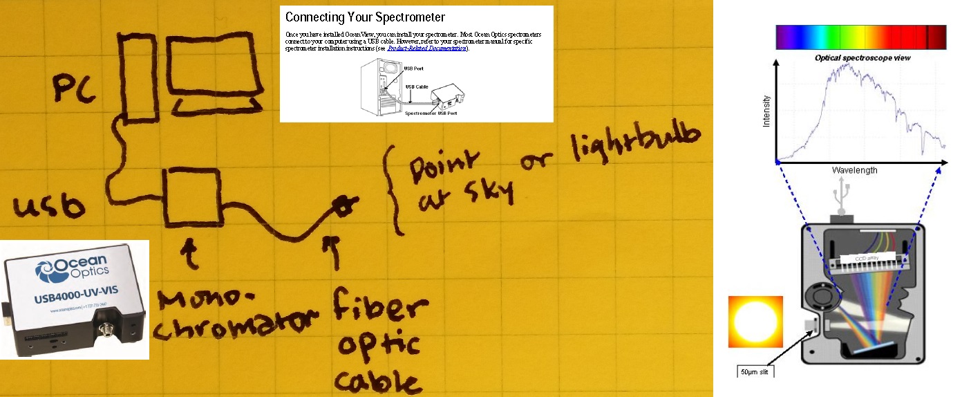
We will use the Ocean Optics USB4000 (or 'Flame', we have 2 different spectrometers) to measure the emission spectrum of two hot bodies, the sun (really the sky), and a hot (light bulb) filament.
Using a multi-mode fiber optic cable that couples light into a fixed grating spectrometer, equipped with a CCD detector, collect as much direct sunlight as possible. Do this for both light sources. The arrangement of the apparatus just mentioned is shown below in figure 3. The student will have read some passages in the manual (pre-lab reading quiz) in order to acquaint the student with Ocean View software.
Figure 3. The Ocean Optics USB4000 set up. We'll actually use an Ocean Optics `FLAME' spectrometer, which is essentially the same as the USB4000. The light source is skylight in the vicinity of the sun. In the second part of the experiment, the light source will be a hot light bulb filament.
The software [2] will allow us to obtain graphs and data files of the spectrum. Be careful to record the filenames. Once you have obtained these data files (bring a flash drive, or email the files to yourself and your co-conspirators), it's all analytical work after that! Once we have collected data files for the wavelength scans for 300-1000nm, you will want to compare the result to that of an ideal blackbody curve as discussed above. Of course there are experimental ``issues'' that one must take care of before one can really make a good comparison. Do the following
Use the software and fiber optic cable to obtain a spectrum of the sky, making sure that the sun itself is not reflected into the fiber optic cable. This spectrum must be all 'scattered light'.
Record the data file with a useful name that will be easily searchable and findable when you search for this data next May. You're going to say, ''why am I am going to do that? I will have aced this lab, long since, and will be doing other things....'' That's probably true. But when you are doing research, you *never* know when you will want to examine data previously taken to help troubleshoot a problem you are having at present. You will then be at the mercy of your previous self, and your commitment to documentation (with sufficient explanation, etc. etc.) and then you'll wish you had kept better records.
Before taking a deep dive into the analysis, use Wien's displacement law (eq. 1) to make a rough the peak wavelength expected of the spectrum you are about to acquire, by assuming (as is commonly assumed) that the temperature of the photosphere of the sun is $\sim 5800K$. Write down what assumptions are entailed in taking this number the blackbody temperature of the sun. Write down your calculation, and your thoughts. This is part of our standard approach: predict, measure, compare while taking data, so that we can be asking ourselves all along, 'does the data make sense?'
Now the rest is analysis:
This is no small part of the lab as you will soon see (in more ways than one). You can see the published spectral response function of the CCD detector grating on our public course website [3]. The curve fitting parameters for this function has been splined with a 5th order polynomial fit of the form \begin{equation}
y = Intercept + B1*x^1 + B2*x^2 + B3*x^3 + B4*x^4 + B5*x^5, \end{equation}
where $y$ is the normalized response function, strictly for
the interval 400-1000nm, and $x$ is the wavelength in $nm$.
Obtain the curve-fitting parameters from the instructors! If only it was a flat function wavelength! But no, it has to be non-linear! I will try to post a file that describes the detector so you can see what I mean. The detector is not uniformly sensitive to all wavelengths of light. So, what the CCD records is actually a distortion of the signal it receives. Not only this, but the grating itself varies with wavelength in efficiency. This too has to be factored in (or out, depending on the point of view). Our simplistic model for the data is this:
\begin{eqnarray}
I_r(\lambda) &=& I_t(\lambda)*ccd_{sr}(\lambda)*gtng_{sr}(\lambda) \\
I_t(\lambda) &=& I_r(\lambda)/( ccd_{sr}(\lambda)*gtng_{sr}(\lambda)),
\end{eqnarray}
where
$I_r(\lambda), I_t(\lambda)$ and the measured and true intensities, respectively, measured as functions of wavelength, and $ccd_{sr}(\lambda)*gtng_{sr}(\lambda)$, are the response functions, respectively, of the ccd and the grating. The operations may be completed in the excel files furnished for this experiment. This statement is also true of our eyes. We will come to this presently. But, to unfold the true(er) signal from the CCD signal, simply divide the received signal by the normalized spectral response function. One can do this by using the spectral response curve fitting function, and evaluating it at every wavelength measured. Replot the two signals on the same graphs. The CCD signal is what the CCD ``sees'', and the unfolded signal is `reduced', by which we will mean something closer to the real signal as it would be measured by an ideal detector. Record your guess: how did you think the reduced signal would look? Hotter or colder? Commit yourself to an answer and record it in your lab notebook.
Plot the 2 curves on top of each other and assess the answer to the question above. Where you right? Explain.
For the solar data, we'll assume the known effective temperature of the sun, $5.8 \times 10^3 K$.
Now plot the theory curve (eq.6) on top of the `true' data curve. You may rescale the peak of equation (the Excel spreadsheet for doing this will be explained in lab; set the variable 'MyTemp' to 5800, and vary the parameter $C_2$, which in the spreadsheet is given the variable name hckb...it should really be hcOVERkb, but that is too weird....) so that the theory curve and the experimental data agree, roughly, around the peak. This will be the primary measurement. Vary the constant $C_2$ for the best fit. Systematically vary $C_2$ over a best range, and from this calculate $h \pm \Delta h$. The uncertainty will be rather big. Our interest is solely in an order of magnitude estimate of the quantity $h$ from a local blackbody radiator. This is the main result of the lab.
Is the percentage discrepancy between $h$ about as big as the percentage
uncertainty, loosely determined from the range of best values of $C_2$? How did you estimate the percentage uncertainty? Furnish quantitative values from your work.
Speculate about the reason for the notches (dips) in the sky spectrum. What physical process can cause them? State your thinking in your own words. These were first observed by Fraunhofer in the late 18th C.
The actual sky spectrum data is systematically below the theory curve in both short wavelength and the long wavelength ranges, on either side of the peak. Speculate about possible physical processes that could account for this. Comment briefly about the implications of these effects on global warming. I will try to have something to say about UV spectroscopy and `vacuum monochromators'. For the longer wavelength stuff, you are on your own.
4.2.1 Task #2: Obtain a spectrum of light bulb, and from its analysis, assuming the accepted value of $h$, obtain an estimate of the temperature of the filament.
Obtain one spectrum for a hot filament, over the same range of wavelengths. Consult your instructor regarding Voltage and Current settings for the measurements.
As in task #1, before taking a deep dive into the analysis, use Wien's displacement law (eq. 1) to crudely estimate the temperature of the filament, now by guessing at the peak wavelength using multiple methods:
look directly at the filament and, comparing the peak wavelength of that light source from the point of view of observed color, make your best guess of the peak wavelength and from it (and Wein's Law), estimate $T_f$, the filament temperature.
The data itself typically shows a peak in the neighborhood of 950 nm. Use Wein's displacement law to estimate $T_f$.
Look up the melting temperature of the filament material. The operating temperature should be less than this, yes?
Consider the consistency of these results and set next to them and sort out whether they are consistent results that permit convergence to an estimate of $T_f$ or not.
Evaluate the significance your calculations, and record your thoughts. This too is part of the standard approach: predict, measure, compare. While taking data, we can always be asking ourselves, 'does the data make sense?' Sometimes it's our 'sense' that is the problem.
Now perform the same data reduction as the the sky spectrum with this difference: take the 'known value' for $C_2$, and vary the filament temperature to obtain a best fit. What's the best estimate of the filament temperature? With what precision do you know it? Now use the Excel spreadsheet to fix $C_2$ to the known value , and to systematically vary 'MyTemp' to obtain the best fit for the filament temperature. This is the second most important result of the lab. Again, what we are after is pretty crude, we just need to answer a question about an inequality, not a precise value.
Record your subjective estimate of the color of the filament. Estimate its uncertainty. How certain are you about the answer to the research question? Is that the same thing as the uncertainty in $T_{f}$?
How is it that the filament looks like the color of the sun, even though it is less than 1/2 the temperature of the Sun? Explain. Hint: you will need to consider the biophysics of the retina as a spectrum analyzer of sorts! Is it? What properties of the instrument we are using for detection come into play here? Do our eyes have similar 'instrument properties'?
References:
From Nobel Lectures, Physics 1922-1941, Elsevier Publishing Company, Amsterdam, 1965. Nearly all the Physics Nobel Prize talks may be read here.
The manual for the device and the software is posted on our public course web site.
See also "CCD spectral response function'' on our site.