4 Wave properties of light, or, how to measure the wavelength of laser light with an actual ruler :) Draft version 3.2...I'll try to get the rest of the typos out before lab tomorrow morning....
The two research question for these experiments are:
what is the wavelength of the laser?
will you avoid looking along the laser beam into the laser itself?
The second question obviously should be answered in the affirmative, but will require vigilance. Pay close attention to the pre-lab technical details shared by the instructor. It was added also to avoid having a one-item list. But really this lab is about measuring the wavelength of a red-ish or green-ish laser using N-slit gratings (2 different ones), and with a ruler. In your abstract, the final sentence (or first) will be something like "the wavelength of the laser was found to be $649.7 \pm 0.3 nm$, using diffraction effects..." or '' $653 \pm 6 nm,$ '' or some such thing. How precise a measurement can you make? Document your work. These two approaches (task #1, use a multiple - slit apertures, task #2, use a ruler) may be used in any order. [Note, that comment depends on the room assigned...Sp25, we will separate tasks #1 from task #2, and do the experiments over 2 consecutive lab periods).
Task #1 : Determining the wavelength with using 2 different multiple slit diffraction apertures (choose 2 of 2,3,4 or 5 slit patterns, but everyone does the 2 slit...)
A collage of pictures related to the set up is shown below, for 2 slit diffraction. We should have a ``Diffraction slits'' accessory wheel mounted on an optics bench
along with a red diode laser set up, as shown below in figure 1. The interference pattern for two
slits is shown below. Note how the single slit diffraction effects
are present in this case as it is for all multi-slit diffraction patterns.
The multi-slit interference intensity peaks are `modulated' by the single slit
diffraction pattern. It's a complicated pattern. Patterns like these will be exploited to make measurements leading to a determination of $\lambda$ for the case of N-slit gratings where $N\geq 2$.
Figure 1. (a) A collage of images depicting the set up: what determines the angle $\theta$ so often used to predict the location of interference maxima? (b) Actual laser light (He-Ne laser?) intercepted by a screen some distance from narrow rectangular apertures. (c) Picture of part of the set up
Where the `small angle approximation' prevails (i.e., $d \ll D, \longrightarrow \Delta l \approx d\sin{\theta},$ where $\Delta l$, is the path length difference between adjacent phasors arriving at the same place on the screen....), the simplest physical model is given by
\begin{equation}
d \sin{\theta_n} = \left\{ \begin{array}{rl} n \lambda & \mbox{n=0,1,2,3,...CI }\\
(n+\frac{1}{2})\lambda & \mbox{n=0,1,2,3,...DI}
\end{array} \right.
\end{equation}
You must now consider whether, given the parameters of your set up, this approximation holds, and what exactly must be measured in order to calculate these angles and so to infer $\lambda$. Further, how can we use this ''physical model'' to obtain a ''computational model'' from which we can obtain a wavelength as a fit to the data. Do the following
Make a cartoon of the measurement system (e.g. `picture' $d$, $D$, $y_n$, etc.) visually defining the variables used in the model, noting how everything is measured along with its uncertainty (explaining how that is estimated....). Measure, record everything you can before turning on the laser. That's just a safety thing.
Read off $d$ from the accessory wheel itself, the distance between the apertures, the width of the apertures, and so forth--do write that down, being keen to record all the information).
In the foregoing, we made reference to the small angle approximation. Does it apply in the set up you have in the lab?
What measurements will you make to arrive at the angle $\theta$ associated with the (principal)
distance between the slits?
record the wavelength of the laser found on the laser itself. Are there serial numbers for the laser, the power supply? Record these.
Anything you measure must have also with it an estimate of it's uncertainty, including a brief rationale for the that estimation. Make sure that all the measurements appear in or near your sketch.
Dial up one of your chosen patterns. The following will suppose you have chosen $N = 3$. Turn on the laser to observe the pattern to get a feel for how far apart the interference maxima are, and what we can use to measure them, and how we'll (you'll) measure them. Before making quantitative measurements, comment on the overall structure of the pattern. You discover that not all the maxima are equally bright as there are now multiple minima in between the principal max's, unlike the 2 slit pattern. The principal maxima are much bigger than the little ones (secondary, tertiary, etc.) in between the minima. This is a qualitative thing. We will come back to this presently.
Before you have taken many measurements, take one of them and use your model, your principle of calculation, and calculate $\lambda$. This is a check on progress. This probably sounds pretty vague. To give better structure, see if you can take one of the principle maxima, it's measured displacement from the center of the pattern, and from it (much like homework problems you have done) calculate $\lambda$ from Eq. (1). Further, estimate the displacement from the center of the pattern to the first diffraction null! These zeroes are associated with the physical model $a\sin{\theta} = m \lambda$. Can we estimate (calculate) the wavelength (however crudely, document how crudely) in the same way? Do this too. Calculate the discrepancy and compare it with the uncertainty of the this single measurement. We want to compare this uncertainty (later) with the uncertainty gotten from fitting all of the data to a theory curve. Once this is done, get as many measurements of the maxima that you can. You will be filling in a table with 3 columns, the thing that will by taken as the independent variable in the modeling plot, the dependent variable (the thing you are measuring having to do with principal max's), and the uncertainty in it.
Using FITTEIA, plot a modeling curve to fit the measured maxima for which the wavelength is a fitting parameter. Recall that the formula will need to be input using a function written in C. If one uses $y = b*x$, where $x$ is the diffraction order, say, and where $y$ is whatever it is, how is $b$ related to the wavelength $\lambda$? Obtain a best estimate of $\lambda.$ It is important that the mathematical model we adopt in this case is one in which $\lambda$ itself is a fitting parameter. Figure out how to write the fitting function in C appropriately. The Goldilocks plot will help determine the uncertainty in this fitting parameter. This is now a separate estimate of the wavelength, using all the data at once, not just an individual measurement. Is this better than a single estimate of $\lambda$ done many times for a single principal max? How; why? Record your thoughts on this. Print the modeling graph(s) and tape these into your note book. One now has a 'best' measure of $\lambda$, with its own uncertainty. Comparing these with the manufacturer's values (that's the discrepancy).
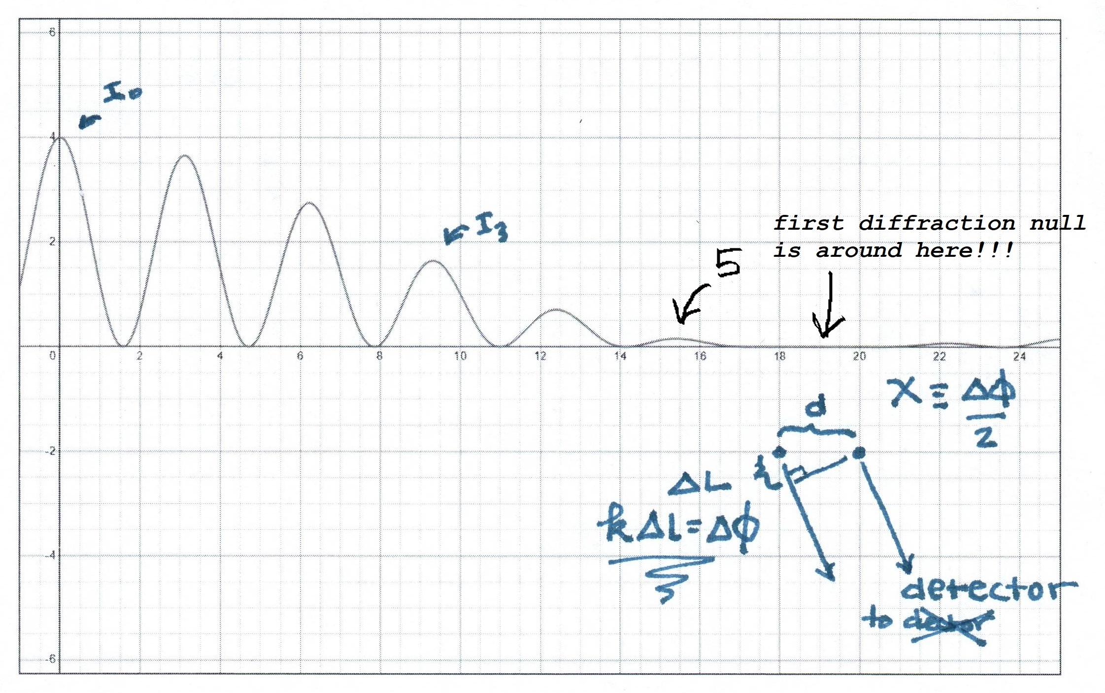
Let's return to the qualitative intensity pattern observed. In the steps above (7?), you have created a qualitative sketch of the pattern, being careful to get the sketch of primary and secondary maxima, and minima, qualitatively correctly. You described qualitatively how the intensity varies from the center to the wings on either side. If you haven't written down your verbal description of the sketch, do this now, BEING CAREFUL TO COUNT THE NUMBER OF N-slit (whatever N is) principle maxima that you can observe under the diffraction envelope. This is a study in description, and can be an intermediate check on progress! How many do you predict there to be? I include a Desmos plot as an illustration for a 2 slit pattern for which $\lambda = 550nm, \: D = 1.64m, \: a = 0.150mm,$ and $d,$ the distance between
the two slits, $0.9mm$. Here we count 5 maxima underneath the diffraction envelope, not counting the central one, or 11 counting both sides including the central one. Is this the count we expect theoretically (according to the physical model)? Explain! Of course our simplest model does not include single slit diffraction effects. But let's now pursue this!
Figure 1.5. A two slit pattern for which we find 5 2-slit maxima underneath the diffraction envelope.
The wave 'model' that yields a prediction for the details of the shape of the intensity pattern (e.g. as in Fig 1.5 above for $N = 2$) falling on the plane that intercepts that pattern is exhibited below. Using DESMOS or fooplot.com, plot the model pattern,
\begin{equation}
I (\theta) \propto \left(\frac{ \sin{ \left(k\frac{a}{2}\sin{\theta}\right) } }{ \left( k\frac{a}{2}\sin{\theta}\right) }\right)^2
\left[ \frac{ \sin{\left( N k\frac{d}{2}\sin{\theta} \right) } }{ \sin{ \left( k\frac{d}{2}\sin{\theta} \right) }} \right]^2
\end{equation}
and compare. How to do this? If you defined \begin{equation} x \equiv \frac{\pi d \sin{\theta}}{\lambda} = \frac{\Delta \phi}{2}, \end{equation}
you could then write \begin{equation}
I (x) = \left( \frac{ \sin{ \left( (a/d) \cdot x \right) } }{ \left( (a/d) \cdot x \right) } \right)^2 \left[ \frac{ \sin{\left( N \cdot x \right)} }{
\sin{ \left( x \right) }} \right]^2, \end{equation}
where $a$ is the actual slit width, $d$ the actual distance between slits. Look up the values on the Pasco Multiple Slits wheel or in the Pasco Precision Diffraction Slits Manual [2]. You'll need to choose a wavelength of course, so use the one written on the laser if there is one, and plot the result
of Eq. 4, comparing the results to your sketch in item (7) above. Be careful to note whether the number of N-slit maxima found underneath the diffraction envelope is
that same as that which you observe! Do you see the expected number of secondary maxima? Don't forget to record the names of plot files that you create and what's in those files. Include images in the upload!
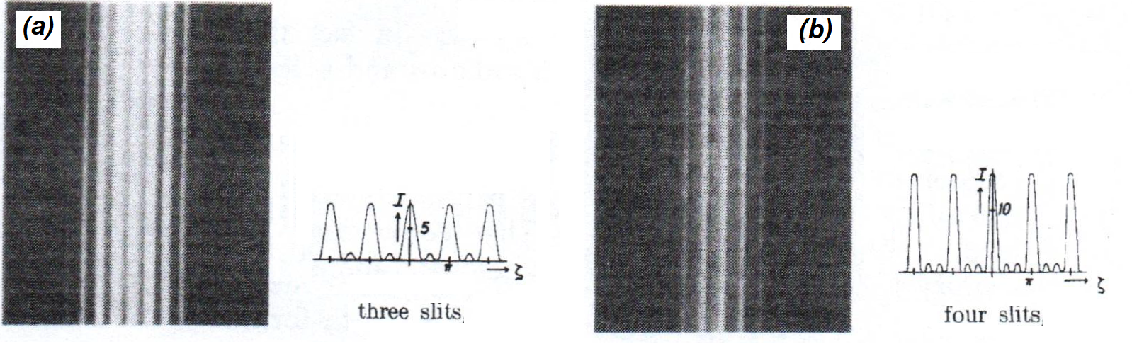
Some examples of real data (with electrons rather than photons!!!) are shown below.
Figure 2. (a) three slit, (b) four slit electron diffraction images, adapted from figures , ``Electron Diffraction at Multiple Slits'',
Claus Jönsson, American Journal of Physics 42, 4 (1974)
Answer this modeling question: are equations (1) consistent with equation (2)? Show that the principal max's of latter lead to relation for the maxima of the former. Hint: the zeroes of the denominator must give us the principle max's. Let's not worry about all the zeroes in the numerator. There's a lot of data there ripe for model comparison, but let's focus on the principal max's. These should be the easiest to see and measure. Once we are done here, write down the principle of the measurement. You are measuring what, for each given what (or for as many as you can), so that you can then calculate.... just a sentence or two.
Use Eq. (2) to model your data for the $N = 2$ case. Compare your results (from best fit values for the fitting parameters) to obtain wavelength given the known values of $a$, and $d$, but why not try modeling all 3 fitting parameters, $\lambda$, $d$, and $a$? Give it a shot. Document your approach!!!
Use the same laser for task #2.
Task #2: Measuring Wavelength with a steel rule: this whole thing will come to tears unless we use steel rules with at least 1/32'' divisions (actual distance between notches---1/64'' is better...), and hey, find that laser you used last week!!! You made a mark on it yes? I will talk to the Lab Manager...the notation should be in the lab notebooks.....
In this experiment you will measure the wavelength first devised by one of the physicist who won the Nobel Prize for the invention of the laser, A L Schawlow [2], but who did not win the patent war for its invention (he was scooped by Gordon Gould who won the legal case with a lab notebook as the evidence of priority, dated and notarized of course). It uses an actual ruler. It also exploits the idea of diffraction from a reflection grating (multiple apertures, not used in transmission, but in reflection, where $N \gg 1$).
Set up the equipment as shown in figure 2 below, right. Schawlow's original set up is on the left, and is discussed in detail in reference [2], but we'll use the set up on the right.
Adjust the ruler so that the beam impinges on the finest scale. Record what scale this is (smallest gap). The steel ruler markings act as
a reflection grating producing a series of bright spots on the wall. The bright spots are the principal max's. The distance to the wall
and the height of the spots can be measured with the the measuring tape and meter sticks. Paper will be provided for your group. Keep it. See if you can tape it into your notebook. If you feel that is too bulky, keep a record of it somehow.
Now the pattern of maxima has changed yet again. What happened to all those lesser maxima and minima that were supposed to be in between the principal max's? This is a modeling (qualitative) question. Write down your answer. Estimate the number of grooved illuminated by the laser, and write this down, explaining how you did it (safely). Use fooplot to aid in generating a plausible answer. Record your thoughts. To aid further in getting familiar with what we'll have to measure, let's analyze the wave 'model' for the case of a reflection grating, for which 'many slits are illuminated'. We follow Schawlow's discussion in ref. [2] to get the mathematical model for the principal max's. It turns out this is easy to express, and once you have stared at it awhile, you will see it is very like equation 1. The incident angle of the laser beam, and diffracted angle shall be called $\alpha$ and $\beta$ defined in figure 2 below, left. These satisfy
the so called grating equation,
\begin{equation}
m \lambda = d(\cos{\alpha} - \cos{\beta}),
\end{equation}
where $d$ is the grating spacing, which is either 1/64" or 1/32", $m$ is the diffraction order (of the principal max's) and
$\lambda$ is the wavelength of the laser
light. Then,
by measuring the vertical displacements from the imaginary plane of the steel
rule projected against the wall, for each order, we may if we wish calculate the wavelength using the grating equation above, or we may make a Taylor expansion (in the limit that $(y_m/x_o)^2 \ll 1$, .... is it??) and arrive at
\begin{equation}
m \lambda \approx \frac{1}{2}d \left( \frac{ y^2_m -
y^2_0}{x^2_0} \right),
\end{equation}
which is the main result of reference [1], and affords a principle of measurement, as well as a mathematical model. The equations 4,5 and 6 (below) all do. The $0$ subscript refers to the `mirror mode' beam (the one for
which the angles of incidence and reflection are the same) in the case
of the vertical displacement, and the distance of the steel ruler to
the vertical plane on which the beams make their image in the case of each
$y_n$. See the figure below, taken from [2].
If, as we will do in our experiment we keep the laser level and tilt the ruler slightly, equation (5) becomes (provided that $(y_m/R)^2 \ll 1$, .... again, is it??)
\begin{equation}
m \lambda \approx \frac{d}{2 R^2} \left( y^2_m -
y_m y_o \right).
\end{equation}
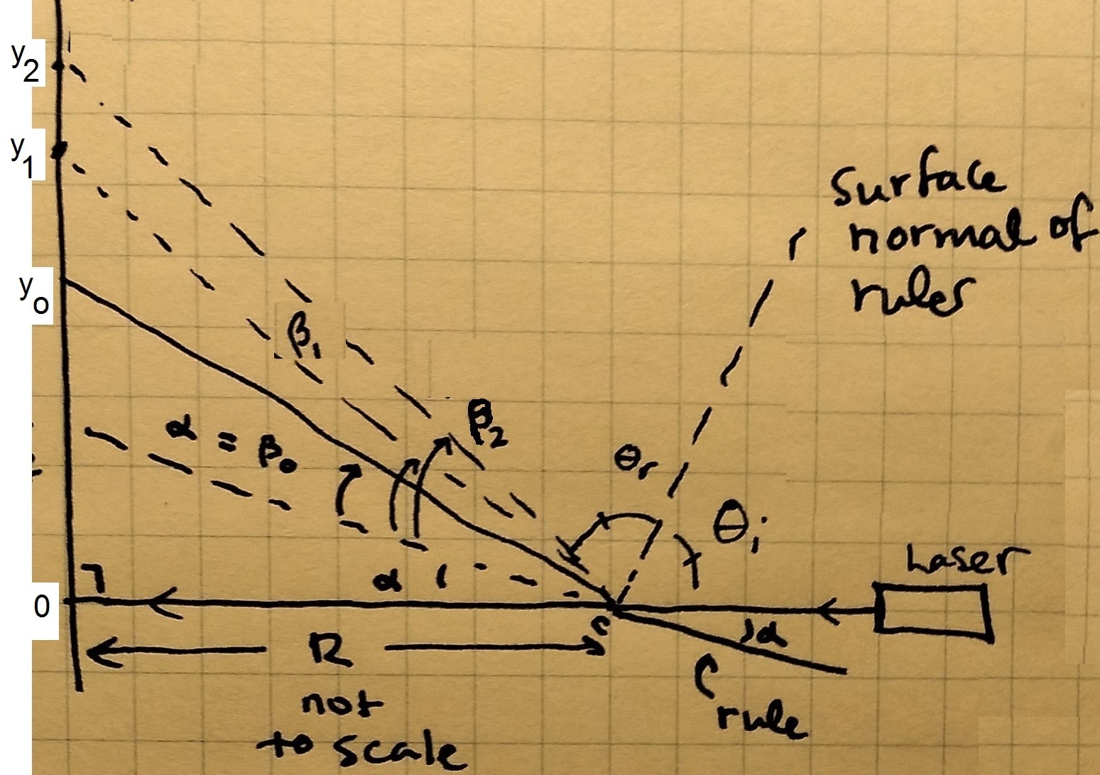
This arrangement is depicted in figure 3 below, right. Sorry about all the scattered notes around the periphery of the figure-it's straight out of my lab notebook. But this is the set up we'll put to use.
Figure 3. On the left, figure 2 from Schawlow's paper, and on the right, same thing, except with the laser leveled and the ruler slightly tilted, as shown. Our set-up is like this one.
Make your own diagram of the apparatus in your lab notebook, introducing suitable nomenclature, indicating what is to be measured to arrive a the necessary values needed to calculate the wavelength. Indicate uncertainties, and write down your rationale for their estimation.
Calculate the ratio $y_m/R$ where $m$ is the largest diffraction order you have measured. How small is this compared to 1? Is the Taylor expansion in equation (6) justified? Exhibit the calculations used to support your opinion.
Contrive to measure the locations of the maxima, and everything else necessary in order to 'model' the expected values for those positions for ready comparison, that is, for an experimental determination of the wavelength of the laser,
$\lambda$. Measure as many locations (of principal max's) as you can. And again, be careful to note experimental uncertainties as they arise, and explain how you estimated or determined them. And as before, before going on too far, 'reduce' one of the $\theta_{max}$'s to a wavelength, just to convince yourself you are on the right track as a check on progress. Quantify the uncertainty and compare this with the discrepancy for this single measurement. Compare this uncertainty (as in task #1) for later comparison with the uncertainty estimated from the fit (Goldilock's style estimation).
Ultimately you will express your answer in the form of $\lambda \pm \Delta \lambda$, where the last term is your experimental uncertainty, gotten from the Goldilocks plot. Make a table with 3 columns, $m$, the diffraction order (principal max's! yes?), $y_m$, the displacement from the central max from the location marked 0, where the undeflected level laser beam would hit the wall), in reasonable units (mm?), and $\Delta y_m$, the uncertainty in that measurement in the same units. Do this for as many max's as possible. It will be useful to create a spreadsheet file (.csv or .xslx, etc.) to cut an paste into the input buffer for the on-line curve fitting interface environment (FITTEIA.org). Name the file and record where it is saved.
Again, using FITTEIA, plot a modeling curve to fit the measured maxima for which the wavelength is an adjustable parameter for the data obtained with the ruler. What fitting function would you use? As in Task #1, it is important to define the fitting function so that the wavelength itself is a fitting parameter. Recall too that the function should be written in C, so that if something is squared, one writes $pow(something,2)$, and if one want the square root of something else, one writes, $sqrt(something\:else)$. Equation (6) is quadratic in $y_m$, the thing one measures with the bright spots on the wall. Aren't there 2 solutions for $y_m$ for a definite value of $\lambda$? Which one should we pick? Solve, and pick one, and so obtain a fitting function for $y_m$, in which the wavelength is a fitting parameter (or the fitting parameter). Obtain a best estimate of $\lambda$, and an estimate of the uncertainty of the method. Use judgment. Explain your reasoning. Print the modeling graphs and tape these into your note book.
This completes the set of measurements of the wavelength of the laser.
How do they compare
with the accepted (manufacturer's) value? Which of the methods do you think is most reliable? Write an abstract quoting your results which compare uncertainties and discrepancies, which uses significant figures appropriately, which captures the essence of the methods, and which interprets what conclusions are supported by your work.