This lab explores how mathematical models are used to compare with experimental data, using the computational tool, ``FITTEIA''. We will use Fitteia to a) make plots of theoretical models and data, and b) determine how well a specific theoretical model `fits' the data, quantitatively. This laboratory exercise will help you become familiar with the tool (Fitteia) that we will use (more or less) throughout the semester to help us compare theory and experiment meaningfully.
Here are two questions important for experimental science classes such as this one to mull over:
Why do experiments at all? What role do experiments play in making science certain?
In what ways can one use mathematical models to analyze results of measurements? What can we learn from this endeavor?
We will discuss these briefly as we begin our work this semester.
What follows is a set of steps to perform to guide us through our exploration of the tool, using a very simple data set.
Create a heading in your lab notebook for this lab excercise, something like 'Fitteia Exercises'.
Go to Fitteia.org, and register. Get (create) your login credentials and all that.
Figure 1. Web page (landing page) for Fitteia
Watch the short instructional youtube video found in the GETTING STARTED menu.
Download and read section 1.3 of the document 'ejp485119suppdata.pdf' Ref[1] at bottom of this page). It is about the The fitter module. Make notes in your lab notebook about things you'll use a lot but maybe will forget next time you login. For instance,
how to enter a formula in the language 'C' (native to, coding used for input to Fitteia) that produces the formulas '\(x^y\)' and '\(\sqrt{x}\)'?
describe the purpose of the 3 main sections of the fitter module.
Login
Click on the Tutorial1 directory. Now you are looking at the web page for the fitter module. There are lots of data sets (files) in the subdirectories that have useful examples from which to learn.
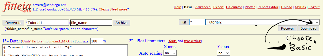
Click on the drop-down menu on the far right of the web page header (see below)in the upper most section, in the so-called web page header, and choose the file named 'Basic', and then click on Recover. This will load the example data into the fitter module sections.
Figure 2. Web page header for Fitteia, a little scrunched up
Create a data table of your own using the data found in the Fitteia buffer. There are only 4 data points so it won't be hard: make column headings for the \(x, \: y, \:\) and \(\Delta y\), the experimental uncertainty (called 'ey' in the data buffer). Create for yourself meaningful table headings, that is, meaningful (descriptive) heading titles, and units for each of the headings. Propose a physical model that accounts for the theory curve, including a column for the mathematical model equation (you can called this the `computational model') and another column for a brief description of the physical model from which this computational model might arise, perhaps and equation of a physical law (e.g. Hooke's Law, F = -kx, etc.). You will have to invent this. This will require both critical thinking and maybe some whimsey. I won't give guidance about the units you make up or which laws are truly pertinent. This is fake data and we are going to try a bunch of different models to see what works best. Call this Table 1.
Click 'fit' next to 'plot'. A linear fitting curve (this is our computational model) appears, or should appear. The linear fitting equation, or default computational model in this case, is of the form \begin{equation} y = a + b*x, \end{equation} where the constants $a$, and $b$ are 'fitting parameters'. Fitteia is written so that the `goodness of the fit' calculation, the $\chi^2$ statistic, is automatically displayed.
It's understood that the computational model will have ``fitting parameters'' that Fitteia systematically varies,
obtaining the value of $\chi^2$ for each value of the fitting parameter. The analysis that is done computationally for is is to find those values of the fitting parameters for which $\chi^2$ is minimum (i.e. the ''goodness of fit'' is best).
No programing is required on your part, except to furnish an equation (the computational model) used for the modeling in `C'. The $\chi^2$ statistic, is defined in [2] (Eq. 12), as follows,
\begin{equation}
\chi^2(p_1, . . . , p_m) = \quad \sum^N_{k=1} \frac{\left( y^e_k - y^t_k(p_1, . . . , p_m, x^e_k)\right)^2}{\left(\sigma^e_k\right)^2},
\end{equation}
where $y^t_k(p_1, . . . , p_m, x^e_k)$ is the value of the model equation calculated for the experimental value of the independent variable $x^e_k$, the `$m$' model parameters are $(p_1, p_2, ... p_m),$ the actual $N$ measured data points are $(x^e_k, y^e_k \pm \sigma^e_k)$ (for the $k_{th}$ measurement), and the uncertainty of each measurement of the $k_{th}$ measured value $y^e_k$ is uncertain by $\pm \sigma^e_k.$ This is a lot to take in. It's kinda like a 'minimization of least squares' but, crucially, includes the experimenter's estimate of experimental uncertainty for each data point.
NOTE: the 'Plot Settings' section (\(2^0\)), controls what this plot looks like! At any rate, you should see a linear fit of the data appear in the plot, with the \(\chi^2\) statistic calculated under the heading 'Fitting results'. This fitting results from a pre-populated function (we are calling this the computational model) in 'Function and Parameters' section (\(3^0\)). We use Fitteia to obtain the plot of the data, with error bars, with the model fitting curve on top of that for visual comparison, the \(\chi^2\) statistic giving a measure for of the goodness of the fit: this is what we want. This is what we are after. Doing this permits you, the modeler, to make an informed statement, an evidence-based statement, a scientific statement, about how well model fits the data. This is what we will try to do for each lab. Note too that the reduced chi2 statistic is related to the chi2 statistic as follows, \begin{equation}
\tilde{\chi}^2 = \frac{\chi^2}{N-M}, \end{equation}
where $N$ is the number of data points being fitted, and $M$ is the number of fitting parameters (also called 'degrees of freedom'). A good fit is one in which the reduced chi2 statistic is close to 1 (not 0).
We will now try two different computational models in search of the computational model that works the best.
In your lab notebook, create a new table to compare hte goodness of fit for the three different models. Choose as column headings, 'Computational model', '\(\chi^2\)', '\(\tilde{\chi}^2\)', 'comments regarding goodness of fit'. Use words to evaluate the goodness of the fit. Is it a good fit or a bad fit? Also, and perhaps most importantly, add a fifth column, 'Physical Model'. Under this column, include the best values of the fitting parameters and their uncertainty, but also a a comment or equation defining the fitting parameters in terms of the variables of the physical model. For example, perhaps 'a' corresponds to 'k' or 'k/m' in the Hooke's law physical model (if that's the one you chose). It will take a little algebraic reasoning to determine this, and do write this down (capture it) in your lab notebook. An example of the top row of a previous student's submission is shown below, which I thought was pretty good. It's not about neatness really but about whether everything required is there....this could've been improved by including an equation defining what 'a' and 'b' are in terms of the variables of the physical model. Do your best. We will develop this line of analysis as we go along this semester.
Figure 3. I thought this was well done, although I would've liked all the physical model information to be in just one column....A well labeled table can show off the results of very complex experiments at a glance!
Click on 'PDF report' (you'll find it underneath the plot, which is above section \(1^0\). Save and rename the output with a meaningful name with your initials at the end, preceded by an underscore, (e.g., weirdfitting_gds.pdf). Make a record of this in your lab notebook (filename, what's in it, etc.)
Obtain this plot for your records for each of the model fits that you try (3 I think).
Now let's try as simple, algebraic, nonlinear model. Edit the Function buffer there in section \(3^0\), and try a square root fitting, and include an off set! Perform a square root fitting (recall, it must be written in 'C'). Make it the functional equivalent of \begin{equation}
y = a + b * \sqrt{x},\end{equation}
where \(a\), and \(b\) are real constants. And then,
Obtain results, evaluate, and fill in next line of Table 2. Note that this includes a verbatim statement of the computational model, etc.
If instead you used, \(y = a + \sqrt{b*x} \), would the value of \(b\) be the same as above, the former case? Would its units? Record your ruminations directly in your lab notebook. It is your diary, record, external brain, your interlocutor, this lab notebook. In a way you are talking to your other self, or maybe to the next student who will do this work, with only your lab notebook as a guide. Anyway, Use the results of your work to complete a second line in your second table.
Continuing, maybe the square root thing is not as good as it gets. Let's now try a transcendental function. Edit the computational model again to perform the fit, \begin{equation}
y = a\sin{(bx)} \end{equation}
where the real constants \(a, \: b \) are fitting parameters. Obtain results, evaluate, and fill in the final line of Table 2.
Ok, one last test. Investigate what happens to the goodness of the fit (magnitude of $ \tilde{\chi}^2$) as the size of the experimental uncertainty is varied.
Let's go back to the square root fit, and let's try it with, well, 5-10 different values of \(\Delta y\). You choose, some smaller, some bigger. Again, use your free will and try stuff. Look at the plots you get for each one, and then
start a new Table (Table 3, the last one...) with the same headings as table 2, but, add a column for \(\Delta y\). You know what? Just do this for ONE of the computational models, not all of them. You pick. Take one of the rows from Table 2 and let that be your beginning for Table 3, adding a new column for and \(\Delta y\). Systematically vary the size of the error bars in the data set, and study how $\chi^2$ and $\tilde{\chi}^2$ vary. Obtain a new result, trying a bunch of values bigger, and a bunch of values smaller than the value that came with the Basic data set.
Make a new data set from Table 3 which plots \(\tilde{\chi}^2\) vs. size of error bar. Is there any uncertainty in \(\tilde{\chi}^2 \)? YES! However we won't pursue that in this lab.
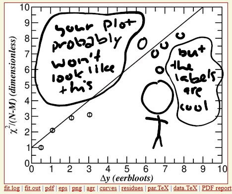
Make a plot of \( \tilde{\chi}^2 vs. \Delta y \). The hard part here is finding out how to produce Greek characters in the axes labels, or, you can totally wimp out and just use English -- however, you will need to indicate units. For help, look for 'fonts' in section 2 of the fitter module, right next to '\(2^0 Plot \: Parameters:\)'.
How do you know the data you have plotted here is any good? This won't seem much like an 'intermediate check of results' or an application of a `predict-measure-compare' cycle that we will be talking more about during the semester. But, write down in your lab notebook what you think would be a reasonable shape for this particular plot. It doesn't have to be detailed. Just answer this question: would \(\tilde{\chi}^2\) be an increasing or decreasing function of the magnitude of the error bars? Write down your thinking. Discuss it with your lab partner. Then, after that, have a look at the plot and discuss whether it make sense or not.
Figure 3. A plot just to exhibit Greek characters in the axes labels. Eerbloots are entirely made up, your units will conform to the physical models you describe in table 2.
write an evaluation that is essentially a 'How-To', so that someone following your procedure can get your results, including a discussion of which model best fit the data drawn from examples of actual physical models taken from PHYS 270 and PHYS 271 that could plausibly apply to such a data set, and details about how one can define the computational model in terms of the natural variables used in the physical model or theory.
upload page images of your lab notebook entries (comments and knowledge capture stuff, responses to questions, etc.) and plots, all bundled into a SINGLE PDF FILE on CANVAS.
Pedro J Sebastião, ''The art of model fitting to experimental results,'' (2014) Eur. J. Phys. 35 015017
Along with the number of fitting parameters (M) and number of data points (N) enable us to estimate the reduced \(\chi^2\), that is, \(\tilde{\chi}^2 = \chi^2/(N-M)\).
We'll quote it here: What is the meaning of \( \chi^2\)?
It is calculated according to Eq. 15.1.5 of the book Numerical Recipes in C, Second Edition (1992) and according to the CERN library MINUIT minimization routine applied to the \( \chi^2\). For a good fit the value of chi2 should be roughly equal to the number of data points, while a good fit for the reduced chi2 statistic is indicated by a value close to 1. [my emphasis] For a moderate good fit the value can be around the number of degrees of freedom (N_exp_points-M_fitting_parameters). The value of chi2 depends very much on the experimental error values of your dependent variable.