We examine the emission spectrum of molecular nitrogen in the final spectroscopy experiment of the semester. We will use the same experimental set up as Lab #6, however we'll use molecular nitrogen discharge tubes. The homo-nuclear diatomic molecule is perhaps the simplest system in which to test the reach of quantum mechanics to describe collections of quantons; so instead of one atom, we study the quantum rules of engagement for two atoms interacting with each other, trapping each other, in what up until the advent of quantum mechanics was unexplainable, a 'simple' chemical bond. Quantum fluids and solids would be next (many atoms interacting), but such experiments are beyond the scope of this course.
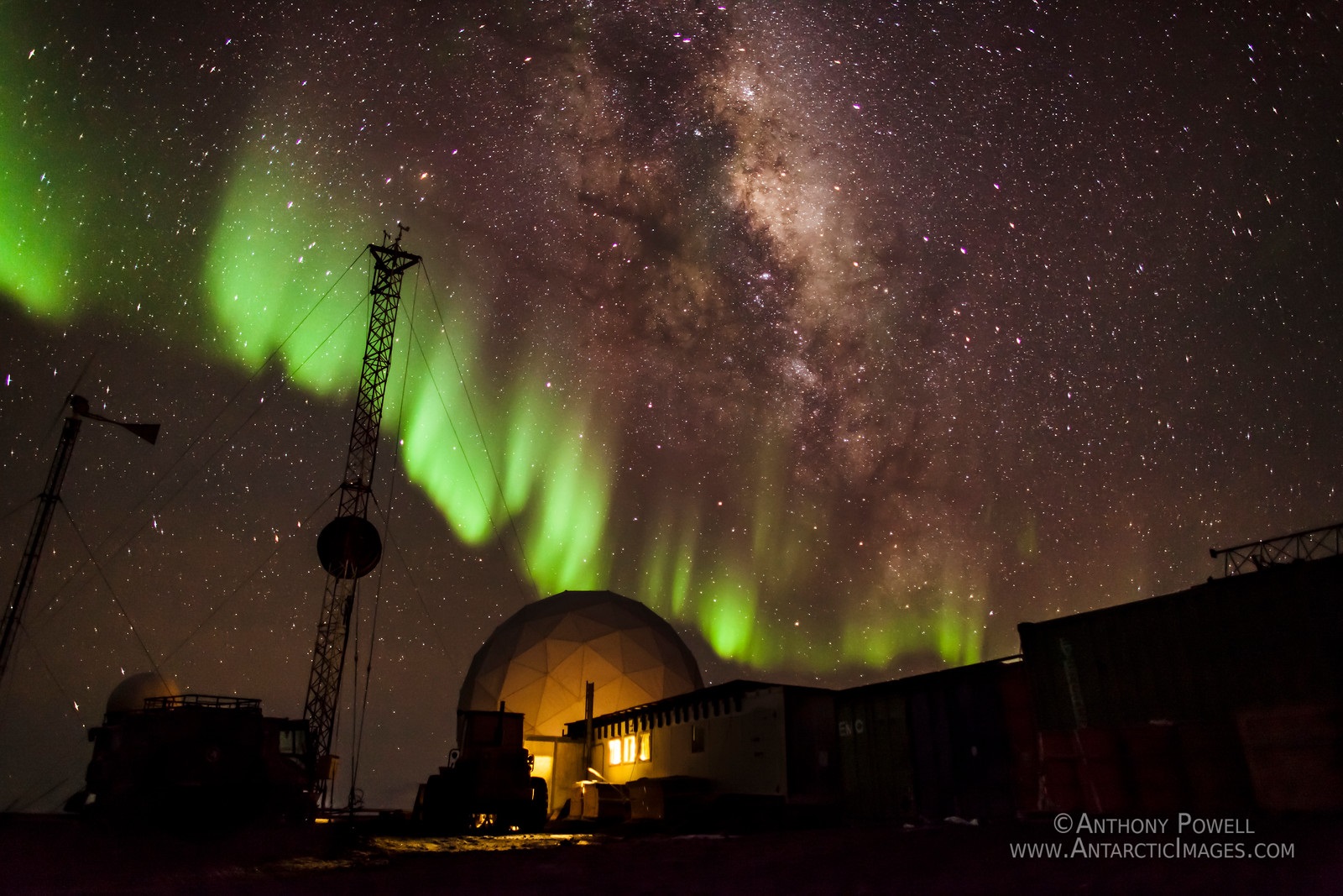
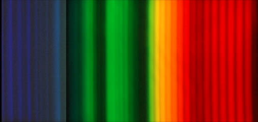
Already with simple molecules we find quantum systems incredibly rich in beautiful phenomena. The most common gas on our planet is not a monatomic gas but diatomic one: molecular nitrogen. Molecular nitrogen is of great importance in atmospheric physics, and one which contributes to the beauty of spaces above the atmosphere (in the ionosphere, typically more than 90 km above the surface of the Earth) in form of the Auroras, shown below both schematically (left), and how they actually look in the wild (middle). The emission spectrum of molecular nitrogen shown bottom right is taken from a Nitrogen plasma in a discharge tube (below, right) such as we've been using in our lab. Aren't the folds of color glorious? Hey, why doesn't our raw data look like that?
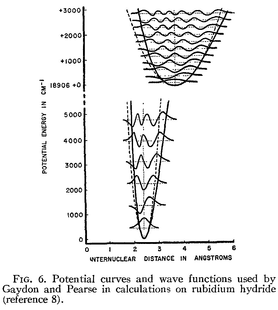
Figure 1. (left) Earth's aurorae, from Discovery ezine, July/August 2017 issue, from the article ``Everything worth knowing about...Auroras''. Note the scribbled in annotation-most of the auroral light from oxygen comes from the atom, while most of the auroral light from nitrogen comes from the molecule. Molecular oxygen is relatively easily dissociated in the upper atmosphere where aurora's live, compared with the much more strongly bound nitrogen atom. (middle left)McMurdo Station, Antarctica, during summer in the northern hemisphere, spectacular auroras abound. Check out the video, 'Antarctica: A year on Ice'.(middleright)A picture of the emission spectrum of molecular nitrogen showing 'band spectra', that is, distinct stripes of color which has stripes within stripes that are too close together for the spectrometer to resolve. The bands themselves are vibrational and the blurry stuff within each band is a rotational spectrum. The different degrees of freedom, quantized, make for a right tapestry of colors, more complex (and beautiful) than atomic spectra!.(right)A picture of electronic states in molecules Rb-H, that create the trapping potential for the nuclei which vibrate in the nearly harmonic trap. The dotted lines show a perfect SHO potential, the solid lines, the actual potential. The horizontal dotted lines show the eigenstates of oscillation for the nuclei, and the wavefunctions are drawn (using the energy level as a proxy for an x-axis!). Each parabolic potential structure is labeled (much like spectroscopic terms in atoms) according to the angular momenta of the electrons, following the quantum rules of adding individual momenta to get totals for both orbital and spin momenta. See the references for a discussion of this!
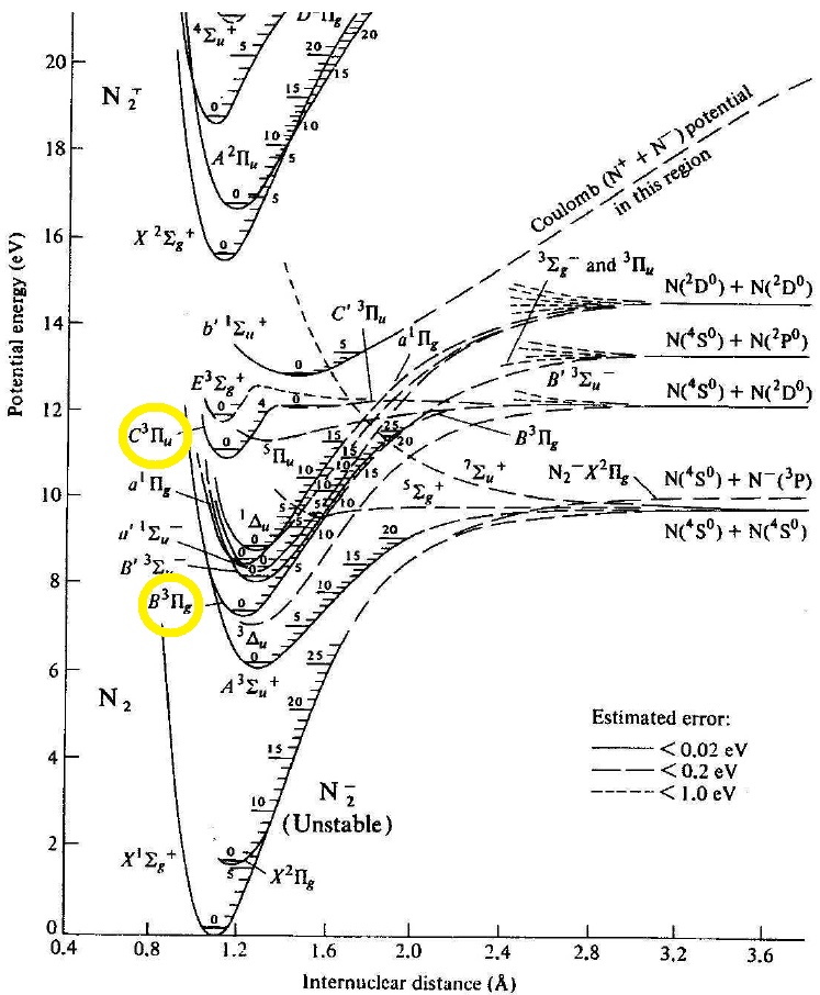
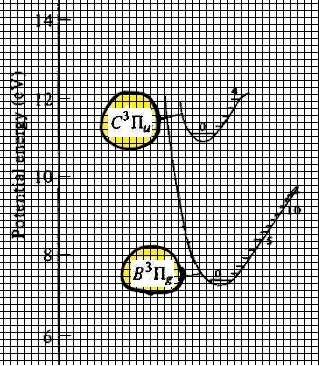
Some of the potential energy curves that confine the nitrogen nuclei and their electrons are shown in Figure 2. We come to molecular spectroscopy expecting that the energy states are straight lines, as in partial Grotrian diagram. Instead we find that each electronic state, or spectroscopic term, is a curve. Almost parabolic, like that of a simple harmonic oscillator. But the vibrational states within each curve is level (monoenergetic). Each spectroscopic term, like that of its atomic counterparts is characterized by a kind of total spin, and orbital angular momentum (e.g. $C ^3 \Pi_u$, where the capital Greek letter stands, as for atomic spectroscopic terms, the orbital angular momenta...don't ask me about the English letter, but in the Greek, you can see a capital 'P' for a state with one unit of orbital angular momentum....the un-gerade and gerade subscripts and the rest of it are discussed in the footnote [1]). In Figure 2, one can see horizontal numbered notches on the right hand inside rim of the confining potential, indicating states of definite (allowed, characteristic, 'eigen') vibrational energies of the molecule within that particular term or electronic state. Note: within a given electronic energy state or term, there are many vibrational states, associated with the quantum number $\upsilon$. The shape of the confining potential is quadratic closest to its minimum, and so molecules furnish a realistic approximation of the ideal quantum simple harmonic oscillator, as mentioned above. Of course the real molecular potential departs from that of the simple harmonic oscillator for a variety reasons which we will not explore except for the first order corrections. One could make a heuristic, classical argument to make the asymmetry about the minimum plausible, but that would be a classical understanding. If we were to take that sort of reasoning seriously, we could not understand how a stable configuration of the atoms the atoms could occur. There is no classical understanding of the (stable) chemical bond.
So, what are the research questions for the experiment?
They are these:
How many transitions can you identify between the vibrational states of two spectroscopic terms, labeled $C ^3 \Pi_u$ and $B ^3 \Pi_g$ (again, see note [1] for a brief explanation of the nomenclature), in the range of wavelengths $350 < \lambda < 500 nm $? Defend, support, explain your identifications in two ways, 1) by crudely calculating the expected wavelength for two of the transitions that you can read right off of Figure 2, as an intermediate check on progress, and 2) by comparing the observed band head wavelengths with the known band head wavelengths tabulated in the literature [2,3]. This question is described with greater specificity in task #1.
What are the values of
$\omega_e$ <\li>
the effective spring constant `$k$', and <\li>
$\omega_e x_e$, the `anharmonicity term', <\li>
for the lower electronic state ($B ^3 \Pi_g$).
Figure 2. Potential energy curves for some of the electronic eigen-energy states (spectroscopic terms of $N_2$, from Figure 1, in Lofthus and Krupenie's work.
7.2 Task #1: How many transitions can you identify between the vibrational states of two spectroscopic terms, labeled $C ^3 \Pi_u$ and $B ^3 \Pi_g$, in the range of wavelengths $350 < \lambda < 500 nm $?
Before getting into the details, let's just say that identification simply means you know how to assign the correct vibrational state quantum numbers for the two states of the transition, the $\upsilon'$ vibrational state quantum number for the upper term ($C ^3 \Pi_u$), $\upsilon''$ integer for the lower term ($B ^3 \Pi_g$). So, what to do?
Obtain a spectrum of $N_2$ in the 350-500nm range, being careful to magnify weak patches (if you need to) by various means available to you. Print these together in your lab notebook so as to form a complete spectrum in the range given. Print a copy of the spectrum or spectra, and affix (tape!). Record in detail the sequence of software commands and settings necessary to obtain and save the data, recording of course the full path names of all files created, with a brief note of what the files contain. This is the raw data. The next few tasks help us characterize it and help us answer this task's question. The peaks you'll see prominently in this range of wavelengths are called band heads. For atomic spectra, the peaks are skinny and symmetric. In molecular spectroscopy, there is an asymmetry about the peak; the intensity gently slopes down on one side and drops precipitously on the other. The gentle slope hides rotational transitions unresolved by the spectrometer we are using. We will not pursue the physics of the rotational spectra even through they are as as cool as they are, and we'll leave the topic there.
What to do with the plot you'll make of the spectrum (saved probably as a .txt file, but plotted with excel, or maybe if you are more daring, FITTEIA...in any case, produce a plot with correctly labeled axes and then...here's what wants to be done:
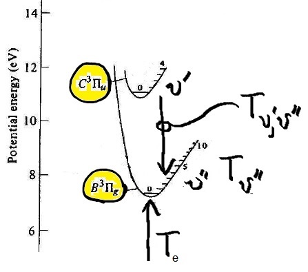
Calculate the expected wavelength for two of the possible $\upsilon'\rightarrow\upsilon''$ visible emission transitions between the 2 electronic states, $C ^3 \Pi_u - B ^3 \Pi_g$, simply by placing a ruler directly on Figure 2, and measuring the vertical separation in mm, say, and from the crude measurement, calculate the expected wavelength with the appropriate conversion factor (e.g., measuring the distance in mm between 0 and 10 eV on the ordinate). Estimate uncertainty for this method, and look to see in the raw data to see whether there is a band head (within the range of uncertainty) at that wavelength. Write down your analysis of this intermediate check on progress in your notebook. The record of what you learned here must be featured in lab notebook. To facilitate this work, see the partial energy diagram shown below. Note that there are tools in Adobe reader that permits you to do this too! But 'analog' rulers are actually even more handy. Annotate the band heads of you have confirmed in this manner. To aid in distinguishing this way of checking results from the next one, please put the vibrational quantum numbers above the identified band head in a box (so for example, over two of the band head peaks there should be something like $\fbox{1'-3''}$, and $\fbox{1'-5''}$, say.
Figure 3. On the left, An edited version of the potential energy curves shown above, highlighting the electronic states, $C ^3 \Pi_u $ and $B ^3 \Pi_g$. A grid has been added to the image to permit the counting of boxes to aid in the calculations. On the right, another image of the same thing, showing the term energy differences for some of the transitions, which for purposes of this lab experiment, we'll define as $T_{\upsilon',\upsilon''}$. For this task however, one can get the energy units directly from the ordinate ('y-axis') units.
Find as many transitions beginning from the upper level $\upsilon' = 1$ vibrational state that you can find in your acquired spectrum, annotating the spectrum itself, and producing a table of these transitions. Look up the known values of the band head wavelengths in Table 29 in the 'nitrogen bible' [2] to identify as many band heads arising from vibrational state transitions of the sort, $\left(1'-\upsilon''\right)$, for as many values of $\upsilon''$ as you can find.
Annotate you plot of the acquired spectrum using proper nomenclature above each identified band head.
Produce a table of results with (at least) 7 columns, identifying 1) the $\upsilon' - \upsilon''$ transition scheme (as is done in table 29 in Lofthus and Krupenie), 2) the accepted wavelength from table 29 (described in the lab handout), 3) the observed value (from the plotted spectrum), 4) discrepancy ($\Delta \lambda_D ?$), 5) experimental uncertainty, ($\Delta \lambda_U ?$), 6) the measured energy gap itself for two of the observed lines, noting that the energy of the transition is referred to as $T_{\upsilon', \upsilon''}$ on our public course web site, and 7) the calculated value of the wavelength from the gap energies (see calculation in the checklist item above. Recall that all column headings must include a meaningful descriptor, and units.
Interpret the degree of agreement between these three indications of band head wavelengths in the usual way, through quantitative comparisons of discrepancy and uncertainty (of measured quantities and their estimates). There is a column for this. Make comments about it.
7.3 Task #2: What are the values of $\omega_e$, $k_{eff}$, and the anharmonicity term, $\omega_e x_e$, for the lower electronic state $B ^3 \Pi_g$?
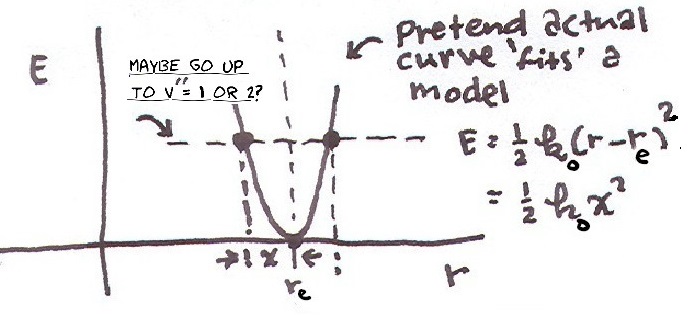
This task quantifies the spacing between vibrational energy levels. The spacing in energy space can be thought of a energy steps. If the trap is perfectly harmonic, with zero anharmonicity, the steps are all the same, a perfect ladder in energy space. But if there is some anharmonicity, there would be a systematic difference between steps. What follows is a description of how to quantify the size of the steps and that systematic difference, the one related to the effective spring constant, and the other to magnitude of the anharmonicity. If the anharmonicity is small then one can estimate the effective spring constant from the shape of potential energy curve discussed above (see Fig. 2). Some nomenclature will help us understand these interrelated terms.
The energy of a vibrational level ($T_{\upsilon}$) in a given electronic state is typically expressed in units of inverse centimeters ($\text{cm}^{-1}$) using the Dunham expansion (Eq. 1).
$$T_\upsilon = T_e + \omega_e (\upsilon+\frac{1}{2}) - \omega_e x_e(\upsilon+\frac{1}{2})^2 + \dots,$$
where
$T_{\upsilon}$: The vibrational term energy, in $\text{cm}^{-1}$. See Table 1 of reference [3], 'Improved fits....'. we find what is meant to be an explanatory master equation for the vibrational state energies for a particular (arbitrary?) spectroscopic term (electronic state),
$T_e$: The energy of the potential minimum, in $\text{cm}^{-1}$.
$\omega_e$: The harmonic constant (related to the ideal spring), in $\text{cm}^{-1}$.
$\omega_e x_e$: The first anharmonicity term, in $\text{cm}^{-1}$.
The naming scheme for the electronic states differs a little
bit from the scheme used for atoms as expected because of
the increased complexity of the system. The ground state
in historical usage is called an $X$ state. The next excited
states are not denoted by 2, 3, 4, etc., but rather by A, B,
C, with perhaps, an $a$ and $a'$, $b$ and $b'$ thrown in. Then,
since the nuclei are in different locations, the neutralizing
electrons do not move in a spherically symmetric potential,
and so there is no conservation of angular momentum in
general. There is instead conservation of the projection of
angular momentum along the axis along which the nuclei
vibrate. These axial components of the angular momenta
for a single electron are designated as before, lz, and sz,
for the orbital and spin momenta, respectively. Delineating
the quantum numbers for angular momenta gets a little
tricky. Capital Greek letters are used to designate the quantum
number number for (the projection of the total) orbital angular momenta. The same sequence of s, p, d, for 0, 1, 2, is used.
The total orbital angular momentum
${\bf L}$ is added to the total spin angular momentum
${\bf S} $ to give the total angular momentum ${\bf J}$, where again,
there are multiple ways in which this needs to be done,
and only the component along the axis along the nuclei
matters, and one sees $L_z = \Lambda \hbar$ and $S_z = \Sigma \hbar$ (and one has to get used to the essential ambiguity in
reference to spin and orbital angular momenta occasioned by the use capital Greek letters, one simply needs to know the context to know which momentum is being discussed). Happily, the total angular momenta is not typically displayed! The total spin multiplicity is also the same as in atomic spectroscopic terms, $2S+1$.
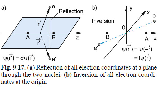
Further, and finally, there are two designation for the spatial symmetry of the wave function that describes the electronic state (the non-spin part), and instead of a superscript there is a subscript, indicating the two kinds of symmetry. Shown below is Figure 9.17 of Demtroder's book Atoms, Molecules, and Photons, (Springer, Berlin, 2005), and is helpful for picturing these symmetries and their designation.
If the electronic state possesses
reflection symmetry about a plane passing through
the axis along which the nuclei vibrate, whether even (+)
or odd (-), this is denoted (sometimes explicitly) by a plus or minus sign as a
superscript, and, further, for the special case of homonuclear
diatomic molecules, there can be inversion symmetry
about the origin (center of mass) which is the same concept as 'parity' in atomic spectroscopic terms. The inversion is simply swapping the sign of all 3 coordinates, or rotating the radial vector by 180 degrees in both polar and azimuthal angles, sort of (see the figure above). States 'even' in this inversion are
said to be 'gerade' and the 'odd' states, 'ungerade', after
the German, for those words, and they appear as subscripts.
This is how spectroscopic terms are composed in diatomic molecules,
Okay? Got it? Easy as $\Pi$.
Also note: in their paper from with Fig1(right) was drawn, the authors Gaydon and Pearse do not label the states! But the modern labeling scheme has a evolved since they published and the foregoing notes attempt to summaritze current practice!