that is, a statistical study of nuclear decay events in $^{210}_{84}Po$ ($\alpha$-decay) and $^{137m}_{56} Ba$ ($\gamma$ decay, with internal conversion electrons )
In this lab the student
will become familiar with the use of the Geiger-Muller tube (GMt)for the detection of nuclear radiation. That's the new technology for this lab. The new physics? It is
the statistics of nuclear counting. That sounds like math, but it's really about the fundamental nature of nuclear decay. Not all nuclei are stable, some spontaneously burst, emitting light energy ($\gamma$ rays), or other energetic particles (e.g., $\alpha$, $\beta$, and neutrons ($n$)). Some of these unstable nuclei are found in the environment in which we live, and some are part of our bodies and have been inside of us as long as we have been alive! Before that! It's not of question of whether you dear reader have been exposed, it's a question of how much. That sounds like a measurement question and that is what this laboratory experiment is about: measurement of nuclear 'radioactive' decay.
<\p>
The student will become familiar with units of measure (the Bequerel, Curie, REM & RAD, Gray & Sievert) and important figures of merit
related nuclear radiation. Do please review Moore's discussions about these matters before lab [1]. Moreover, we will explore the distribution of counts of actual decay events in 2 different limits, limits that frame our experimental research questions. Rutherford [2] described these sorts of experiments as follows (here focusing on $\alpha$ decay),
In counting the $\alpha$ emitted from radioactive substance either by the scintillation or electric method, it is observed that, while the average number of particles from a steady source is nearly constant, when a large number is counted, the number appearing in a given short interval is subject to wide fluctuations. These variations are especially noticeable when only a few scintillations appear per minute. For example, during a considerable interval it may happen that no
$\alpha$ particles appear; then follows a group of $\alpha$ particles in rapid succession; then an occasional $\alpha$ particle, and so on. It is of importance to settle whether these variations in distribution are in agreement with the laws of probability, i.e., whether the distribution of $\alpha$ particles on an average are expelled at random both in regard to space and time. [my emphasis] It might be conceived, for example, that the emission of an $\alpha$ particle might precipitate the disintegration of neighboring atoms, and so lead to a distribution of $\alpha$ particles at variance with the simple probability law.
We need only a few things to define to make sense of this extended quote. No source is 'steady' if the observation time is long compared with the 'half-life' ($t_{1/2}$) of the radioactive nucleus being examined. During such a long observation time, the number of counts will be observed to decay exponentially with the usual form one often associates nuclear decay. Here, the 'short interval' means two separate things: 1) the observation time is broken up into many sampling intervals or bins ($N$ the number of intervals, $\: N \gg 1$) shorter observation times $\Delta t$, such that the sum of which is the total observation time, ($T = \sum_j^N \Delta t_j$) and 2) the shorter observation time itself is much, much shorter than the half-life ($\Delta t_j \ll t_{1/2}$), so short that sum of all of them, the total observation time, is also much, much shorter than the half-life ($T \ll t_{1/2}$)! One of our experiments will satisfy these relationships, these inequalites. The distribution Rutherford had in mind to describe the fluctuations in the counts found in successive counting intervals (the $\Delta t's$) a Poisson Distribution. The second limit is one in which $T \gg t_{1/2}$. We should capture the exponential law in this way.
Our research questions are these:
Which distribution of counts best characterizes the counts measured by the GMt for the $\alpha$ decay of $^{210}_{84}Po,$ when $T = 2000s$, and when $\Delta t = 1s$? Your modeling choices are the Gaussian, and the Poisson distributions. The half-life of this process is known to be 138.38 days.
Do we see an exponential law emerge in the counts measured by the GMt for the $\gamma$ decay of $^{137m}_{56} Ba,$ when $T \approx 1/2 hr.$ and $\Delta t \approx 10s$? And the half-life so measured, how does it compare with the known half-life of 2.55 minutes?
8.1.1 Two notes about Probability distribution functions:
The Poisson distribution function arises from what are called Bernoulli trials, that is, from random events that can have only 2 outcomes, namely that the event happened, or it didn't. The event in question in these experiments is the radioactive decay of an unstable nucleus, and the question is whether a nucleus decays or not during a sampling interval $\Delta t$. Well, OK, it's about all the nuclei in the sample, but it's helpful to think about just one. The probability of recording $n$ counts in any one sampling interval is \begin{equation}
P_P(n) = \frac{e^{-\mu}\mu^n}{n!}, \end{equation}
where $\mu$ is the average count per counting interval, defined by $\mu = N_T/N$, where $N_T$ is the total number of recorded counts over the whole time $T$. Notice I haven't defined the count during the $j-th$ counting interval; what would that be, $N_j$? Anyway, $\mu$ is often (sometimes?) written as $\overline{n}$. The frequency of the number of sampling intervals in which a particular value of $n$ counts is recorded is what is meant by the 'distribution' of counts. If we plotted this distribution, the measured one, we could compare it with the Poisson distribution in Eq. (1) by also plotting $N* P_P(n)$. But we have FITTEIA for this, so we needn't do anything other than prepare frequency data set just described to input as as the data.
For the Poisson distribution, there is a necessary connection between the mean value and its variance, namely, the square of the standard deviation, $\mu \equiv \sigma^2$. The function $P_P(n)$ is defined on the integers, and is often plotted as a histogram, frequency of a given count, vs. counts. The ordinate records how often a given count occurs among the counting intervals, and the abscissa simply enumerates the count itself from 0 to some integer larger than the largest count. A word about the shape of the Poisson distribution function: it's skewed about the mean value, higher on the low side, lower on the high side. See figure 1 below.
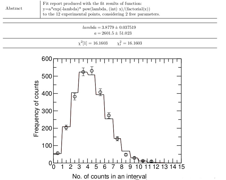
Figure 1. Histogram of variation in number of counts for a Po-210 source, measured by Rutherford et al. [1], as modeled using a Poisson Distribution in Fitteia. This is standard Fitteia output; note the modeling function.
This distinctive skewness can be lost. In the limit that $mu \gg 1$, this skewness goes away and the Poisson distribution becomes symmetric, indistinguishable from a Gaussian distribution function. This is a consequence of the mathematical truth of the Central Limit Theorem, popularly referred to as the 'Law of Large numbers', and is related to ubiquity of bell shaped distributions of measurements about a mean. However, the Gaussian or Normal distribution (there are other symmetric distribution functions, but let's stick with the Gaussian distribution) is not, despite its utility in describing random processes, necessarily, inherently, about random processes. In principle, deterministic processes could lead to such distributions. Deterministic trajectories exist in the framework of classical Newtonian dynamics. But the sheer enormity of trajectories that exist, say, in a mole of atoms in a gas well characterised by a temperature $T$, one 'stoops' to making models with statistical arguments. I said, 'stoops', there in the sense of giving up the idea of calculuating the actual individual trajectories (of all $6.023 \times 10^23$ atoms), not in the sense of doing something unintelligent. The work of Boltzmann is regarded with high esteem by great mathematicians [3]. Had Maxwell lived well beyond his 48th year, he may well have won the first Nobel prize, although most certainly it would've been for his work on the dynamical theory electromagnetic fields. But his work on the application of statistical theories to dynamical systems was also seminal. In any case, the Maxwell-Boltzmann distribution of velocities of a classical gas of atoms in thermal equilibrium at some temperature $T$ is less about randomness and more about making accurate assessments of mean values, their variance, and other 'moments' calculable using the distribution function. In such a framework there is no a priori necessary connection between mean values and their variance. One could easily, for example, have a very cold gas of atoms, or very hot, each nicely described by Gaussians with means that tell us about flow, with variances that tell us about temperature, with no connection between the two. There can be hot and cold flows with the same mean speed, very different flow speeds with the same 'beam' temperature. In any case, to model counts in a counting interval with a Gaussian, one writes \begin{equation}
P_G(n) = \frac{1}{\sqrt{2 \pi \sigma^2}} e^{ -(n-\mu)^2/(2\sigma^2) },
\end{equation}
and one has to separately model the mean and the standard deviation. But as discussed above, in the limit that $\mu$ is sufficiently large, the two distributions become increasingly indistinguishable, the Poisson becomes Gaussian. We shall test this with our data sets.
Finally, if the total counting interval exceeds, significantly, the half-life of the radioactive nuclide, then we can observe the rate of activity decay exponentially down to a background rate, \begin{equation}
R(t) = R_0 e^{-\lambda t} + R_b,
\end{equation}
where $\lambda$ is rate constant characteristic of the nuclide, and related to the half-life through the relation $\lambda = \ln{2}/t_{1/2}$ This will be the case for the Barium decay, in Task #2. Here it will be helpful for the student to review first sections Q15-3, and then Q13-6 in Moore. But first things first:
8.2 Task #1: Count nuclear decay events decay events, $^{210}_{84}Po \longrightarrow ^{206}_{82}Pb + \alpha$, over a total elapsed time much, much shorter than the known half-life (138.4 days) of the sample, and observe, measure, the distribution of counts per counting interval. Which distribution function fits best, the Poisson or the Gaussian?
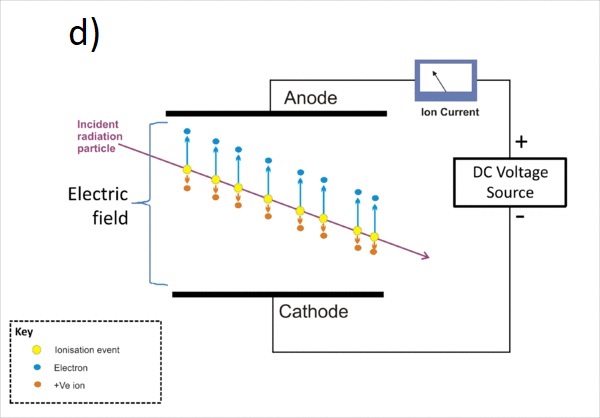
The method we use to count particle emitted in nuclear decay events is the so-called electric method Rutherford refers to above, a gas filled cylindrical tube, well shielded except at its face, with a high voltage pin coaxial with the tube. As an energetic particle traverses the volume, ionization events rapidly occur, and the strong electric field inside the tube causes an electron avelanche to the pin, producing a current pulse which is registered electronically as a count. A species of such a device is called the Geiger-Muller tube (GMt), and we are using one for our experiments, pictured below.
We will use the GMt to obtain counts from 3 sources for analysis:
background radiation
a sealed sample of $^{210}_{84}Po$, (an old one (2017) and one slightly less old (2019), consult with instructor)
Figure 2. The GMt (a) is positioned directly above the source of radioactivity placed in a plastic holder, a few cm. away. An electronic
timer (b) coordinates the counting, and is hardwired to a pc, running software (c) that creates a spreadsheet (a .tsv file) of the counts. The manual for the hardware and the software are found on our public course website (ST260 Manual [4]). A Geiger-Muller tube (d) is also shown, simplified. In common tubes, the anode and cathode are coaxial, with the cathode being a central wire. A current avalanche arising from ionization is collected and forms a single count.
Notes for data taking for each source:
Prepare the GMt for counting experiments. Set the GMt voltage to 770V using the analog knob on the timer itself (figure 1b) so that the tube operates near the so-called plateau regime (see figure 34 in the ST260 manual).
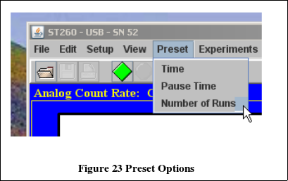
Set the time (duration) of the bins to 1sec, and 'runs' to 2000. Look for the Preset menu item, and set 'time' and 'number of runs', and note the green diamond....in a moment you'll click on that the start the counting.
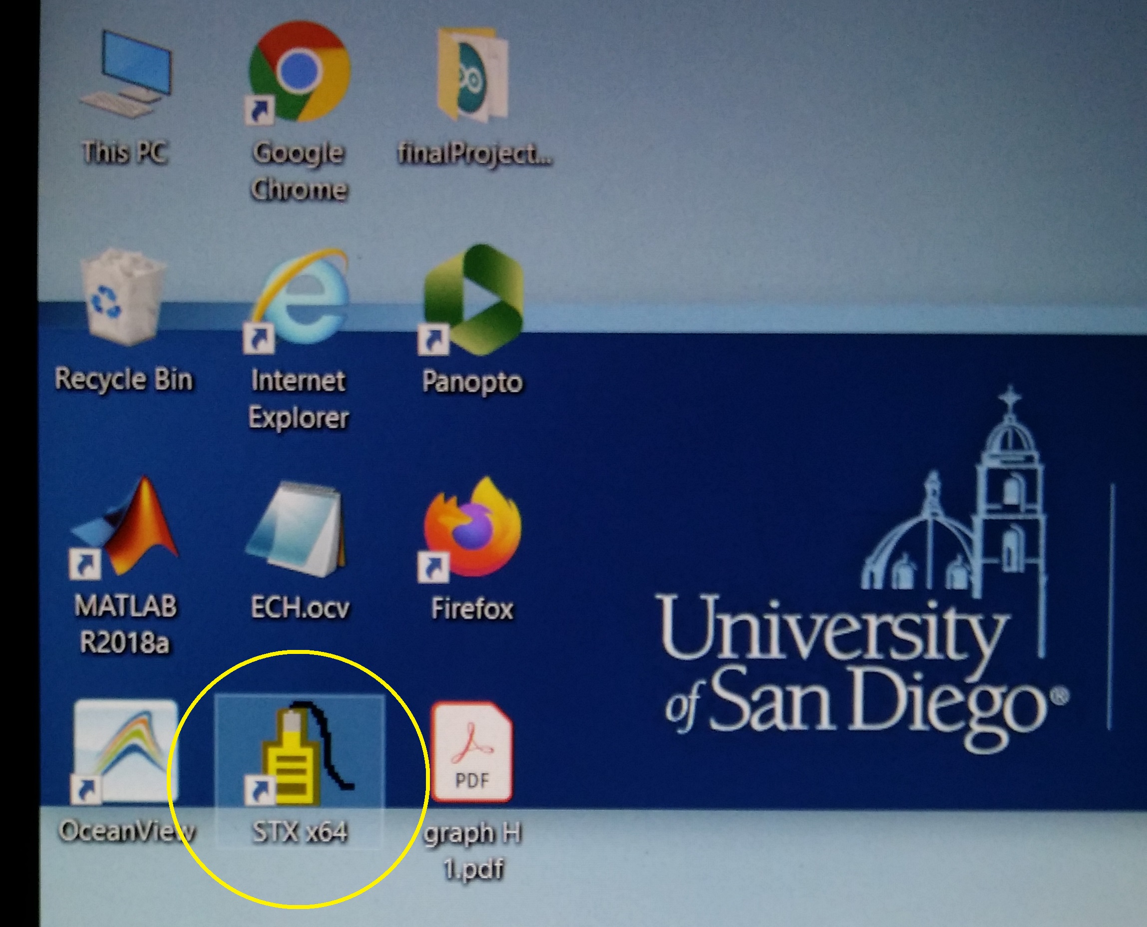
Figure 3. Presets for time (duration of $\Delta t$) and number of counting intervals. Also shown is the left hand side of the landing screen of the our laptops stored in 292. The top secret login information is written in large font on the whiteboard in ST292. You want the icon of the GMT (STX-x64), to wake up the software.
place the source on the top shelf (note: if this is 'background' no source is placed on the shelf) under the GMt, start counting (see above about the little green box) and begin measuring counts. The data will be stored in a .tsv file.
Copy (save) the .tsv file generated by the software to a handy location for further analysis. In your lab notebook, record the chosen file name, what's in it, where it's recorded, and be sure share with members of the team.
The data now will need to be "reduced". By this we mean we need to know the frequency with which a given "count" occurs. This distribution of counts, a distribution function (of counts), is the thing we want to examine to see whether it best matches a Poisson distribution (eq. 1) or a Gaussian (eq. 2). This reduction is easily computed using Excel's Frequency function, an array function, which is executed by highlighting a blank array and entering the key commands, cntrl-shift-enter, altogether at once. Read about this useful function here.
Of course, the best place to learn about it is in the help files in the version of excel that you are actually using.
Calculate $\mu$ in Bq for each set.
Use Fitteia to model the experimentally obtained distribution of counts for each of the sources (background, 'new' Polonium source, 'old' Polonium source, again, consult your instructor concerning the sources available for the experiment) both with a Poisson distribution and a Gaussian distribution. Obtain, quantitatively, the goodness of the fit: this means obtaining the reduced $\chi_{\nu}^2$, that is, $\chi_{\nu}^2 = \chi^2/(N-M)$, where $N$, here, means is the number of data points used in the fitting (just checking in here: is this $N$ the same as the $N$ used in the definition of $\mu$ above???), and $M$ is the number of adjustable parameters. Notice the way in which the factorial is sometimes coded in C in an expression for the Poisson distribution:
using $A$, $\lambda$ and $\overline{x}$, $b$, as fitting parameters. Here, $x$ corresponds to $n$ in Eq. 1, etc., etc. The constant $A$ is an arbitrary amplitude adjustment. Be careful to write down in your lab notebook how the function used (Eq. 4 and 5, or something like it) for the numerical fitting maps in detail to equations 1 and 2. This is part of the 'How-to' thing!
Which probability distribution best fits the histogram using the notion of 'goodness of fit'? A Poisson distribution, or a Gaussian distribution? Discuss. Evaluate. Come to a defensible conclusion and evaluation of this question.
In order to acquire perspective about figures of merit with the respect to the magnitude of counts, to get some idea of what is big or smallm estimate the number of counts in Bq you receive from the $\beta$-decay from C-14 in your own body. This should be, if we do it corrently, 'small', and 'safe', yes? Do the following:
) Estimate the number of C atoms in your body (you have C atoms, about $18 \%$ by some estimates of your total mass)
and
) the number of $^{14}_6 C$ atoms in your body. A standard value for the fraction of $^{14}_6 C$ in a sample of carbon is $1.2\times 10^{-12}$ $^{14}_6 C$ per $^{12}_6 C$ (of course not in dead things....because of the decay rate of $^{14}_6 C$...)
and so
) calculate the present rate of radioactivity of beta decay in your body right now (which has been going on all the while you have been alive). Express your result in Bq.
) Now calculate your annual exposure in mSv (milli-Sieverts). A Sv is Gy (Gray, or energy deposited, in J/kg) multiplied by the RBE, or Relative Biological Effectiveness. The RBE for beta radiation is 1 (for slow neutrons it's 4-5). Compare this result with the average counts (now you can give these with uncertainties as well), and with average annual background radiation found in Table Q15.1 in Moore. Rats, I forgot to tell you the most important things! The energy deposited per each $\beta^-$ decay is listed in several places as 0.1565 MeV!
)Finally, cf. with the accepted annual background radiation in mSv from external sources (of order 1 mSv...). Are you nuking yourself less than annual background sources? Explain.
8.3 Task #2: measure the $t_{1/2}$ of $^{137m}_{56} Ba$ decay, by observing monotonic decay of counts per counting interval, where the sum of the durations of all the counting intervals is greater than the half-life of the sample, and compare with the accepted value for the decay (2.55min).
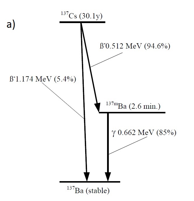
Figure 4. One of the decays exhibited by Cs 137 is the $\beta^-$ decay is to the metastable state Ba 137m which decays 90 % through a .66 Mev $\gamma$ to the stable state $^{137}_{56} Ba$.
What's different in this task is that our sample will be freshly prepared at the moment of use, and the mean count per sampling interval diminishes dramatically with time. Our Lab Manager will prepare the sample using a weak solution of hydrochloric acid. The fluid removes Ba-137 from Cs-137 chemically, suspending the Barium isotopes in solution. Just 5-10 drops of the 'eluting' solution will do. The drops are placed into metal cup (planchet) which is the then set into the plastic sample holder and the counting cacophony begins. The energy level diagram shown below indicates the principle decays, particles, energies, and half-lives. The known half-life is 2.55 minutes. At the end of our work, the student will demonstrate an analysis of counts vs. time measurement that is to be compared with the known half-life. This is one of the principal results of this experiment.
The question of safety from exposure to radioactivity of course arises in t The question of safety from exposure to radioactivity of course arises in this part of the experiment too, although the air layer that protected us from alpha decay is no longer sufficient for the $\gamma$ and $\beta$ radiation generated by Ba 137m (and to a far lesser extent, from the Cs 137). This is worth a longer disc
ussion (taken up in a Health Physics Society post on the very question, see ref. [6]
In more detail,
Set the HV to 770V as we did last time.
Set the time of the bins to 10 sec, number of runs to 250, and begin measuring background counts, while waiting the freshly prepared source. One wants at least 250 runs once the planchet has been received. This is a design choice. Explain whether it is a good design choice, given that $t_{1/2} = 2.55 min.$ Sorry for asking that question with such vagueness. Calculate how many halflives you get with 300 runs at 10 sec per sampling interval, and whether that's enough to reduce the activity of the sample to below background. You will need an initial condition perhaps (counts at t = 0). Let me use history to furnish this. In 2017, the planchets at the beginning showed counts of order 150 Bq. Do the calculation suggested and comment on the design of the experiment. Once you're done with this calculation, you may receive a planchet with the `hot' fluid.
Place the planchet on the 2nd shelf, record counts.
Copy the .tsv file generated, uniquely named, etc., etc.,
Using Fitteia in the usual way (do please record your procedure for preparing files for analysis in detail!), using equation 3. Does the measured half-life agree with the known half-life within error? Explain! Use significant digits appropriately (note that the Fitteia report does not...it's not wrong, but it is extremely unhelpful, and nonstandard in format).
The decay shown above in figure 4, or rather one of them,
\begin{equation} ^{137m}_{56} Ba \longrightarrow ^{137}_{56} Ba + \gamma, \end{equation}
produces a $\gamma$ that inefficiently ionizes the gas in the GMt. A fraction of the time (about $10 \%$), an internal conversion event occurs and an electron is ejected from the atom, one from the inner or lowest atomic energy states, which is then followed by a cascade of x-ray transitions. The internal conversion electron is much more efficient at ionizing the gas in the Gmt. Comment, in your discussion of results, about a possible reason why the energetic electron is more efficient than the $\gamma$ at ionizing the gas.
Do you expect the background counts after the counts have died away to a constant value to be the same as the original (no sample) background count done in task #1? Carefully consider. Be sure to study the SpecTech manual for this particular experiment [5]. If the background count exceeds that measured earlier in the day, what might account for it?
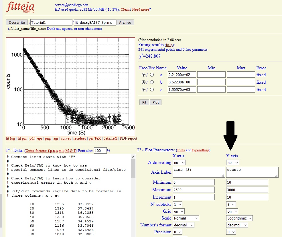
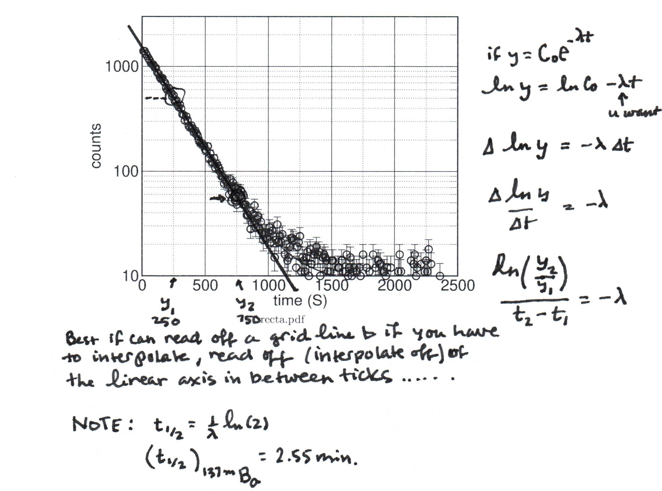
As an intermediate check on progress, set up the Y AXIS parameters to provide a semi-log plot of the raw data, and from the slope, calculate 'by hand' the half-life in minutes. Here follow two pictures that outline the process. Why do this? If one chooses to plot the dependent variable (measured thing) with a log scale but leave the time base (dependent variable) linear, then a process like $y = e^{-\lambda t}$, will appear as a *straight line* on the graph paper! This is what semi-log paper lives for! It says, "let me show you the exponential part of the process you are messing around with here, in this experiment''. It really says that! You can pencil out the half-life; see below.....
Figure 5. Set up FITTEIA Y axis parameters for a `log-lin' plot, and get the coefficient in the exponential from the slope of the semilog plot. About the note in the figure on the $rhs$, the 2.55 min is the accepted value for the Barium decay, it is this you'll use to obtain your discrepancy....when I tried to calculate the value for $\lambda$ for this data set I think I calculated 2.64 min, but I haven't estimated the uncertainty in the slope as of this writing!
Now, the abstract.
References:
Review Q13.6 and Q15.3 in our text. Also, a cool historical survey written by a great nuclear physicist can be found in our 'cool papers' folder,
Bethe, H, `Nuclear Physics'. Merely reading section 1 will be a short, and worthwhile read.
Rutherford, Geiger, and Bateman, 'The Probability Variations in the Distribution of $\alpha$ Particles', Phil. Mag.20, 698, (1910).
See Cedric Villani's essay in the book, 'Boltzmann's Legacy', Yngvason, J., Gallavotti,G., and Reiter,W. L., (European Mathematical Society Publishing House, Switzerland 2008) p.129-144, entitled, "H-theorem and beyond: Boltzmann's entropy in today's mathematics". Cedric Villani was the 2014 Fields Medal winner.